Detached-eddy simulation of supersonic flow past a spike-tipped blunt nose
2018-09-27YuanXUELiangWANGSongFU
Yuan XUE,Liang WANG,Song FU
School of Aerospace Engineering,Tsinghua University,Beijing 100084,China
KEYWORDS Detached-eddy simulation;Drag reduction;Oscillation mode;Pulsation mode;Spike-tipped blunt vehicle;Supersonic flow
Abstract Space vehicle in atmosphere travels mostly at supersonic speed and generates a very strong bow shockwave around its blunt nose.Oblique shock and conical separated flow zone generated by a forward disk-tip spike significantly reduce the drag by reducing the high pressure area on the blunt nose.This study employs improved delayed detached eddy simulation to investigate the characteristic flow structures around a spike-tipped blunt nose at Mach number of 3 and Reynolds number(based on the blunt-body diameter)of 2.72×10⁸.The calculated time-averaged quantities agree well with experimental data.Characteristic frequencies in different flow regions are extracted using fast Fourier transform.It is found that two distinct instability modes exist:oscillation mode and pulsation mode.The former is related to the foreshock/turbulence interaction with nondimensional frequency at around 0.004.The latter corresponds to the interaction between turbulence and shock structures around the blunt nose,with a typical coherent structure shedding frequency at 0.092.
1.Introduction
Blunt body vehicle flying at supersonic speed leads a very strong bow shockwave at the upstream around its blunt nose.The shockwave generates both high drag and heat to the blunt nose.This may damage the nose and equipment it carries.A disk-tip spike is able to generate an oblique shockwave at a distance away from the blunt body and a conical separated flow zone between the disk and blunt nose.As a result,disktip spike can significantly reduce drag by reducing the high pressure area on blunt nose1.
However,the formation of shear layer and recirculation zone in between the spike and blunt nose introduces additional unsteadiness into the flow field,as first reported in measurements in 1950s2–4.Bogdonoff4first observed that there exist two typical instability modes in such flows:the oscillation mode corresponding to the foreshock/turbulence interaction and the pulsation mode related to the interaction between turbulence and shock structures around the blunt nose,as illustrated in Fig.1.The mechanism of oscillation mode was explained by Feszty et al.5through theoretical analyses while the one of pulsation mode was described based on several hypotheses.6,7
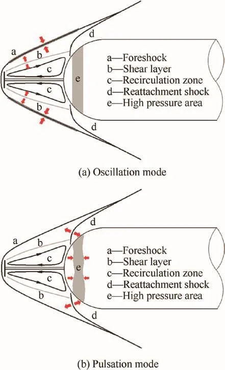
Fig.1 Sketch of typical instability modes of flow field around disk-spiked blunt bodies.
In 2011,Ahmeda and Qin reviewed the progress and state of the aerothermodynamics of spiked supersonic/hypersonic vehicles.8They claimed that compared to the large amount of literature on parametric studies for engineering applications,numerical investigations on detailed flow physics were relatively rare.To date,the numerical simulation techniques are limited to steady or unsteady Reynolds-Averaged Navier-Stokes(RANS)methods.9
The high-speed real-geometric cases present ideal applications for Hybrid RANS-LES Methods(HRLM),because of the well-known limitations of RANS approach in the context of unsteady separated flows.Besides,the use of Direct Numerical Simulation(DNS)or Large-Eddy Simulation(LES)10costs huge computer resources with little accuracy increase in the prediction.
The first HRLM,Detached-Eddy Simulation(DES),11benefits from the advantages of RANS at near-wall region and LES elsewhere.Then two improved DES variants,DDES(Delayed DES)and Improved DDES(IDDES),have been further proposed by,respectively,Spalart et al.12and Shur et al.13The ability to capture massively separated flows with affordable computational cost has prompted their use over a wide range of application areas.
The present objective is thus to numerically study the unsteady turbulent flow structures around the spike-tipped model of Gnemmi et al.,14by using the IDDES method.Shear Stress Transport(SST)model15,16is chosen as the underlying RANS model.To the best of our knowledge,the present IDDES calculation makes the first try on such lf ows.
2.Numerical methods and grid generation
2.1.Flow solver
All computations are carried out with an in-house code that solves the compressible Navier-Stokes equations on multiblock structured grids.The standard Roe’s Flux Difference Splitting(FDS)scheme with 3rd-order MUSCL extrapolation is adopted for inviscid- flux approximation,whereas a standard central scheme for viscous flux terms.A 2nd-order backward difference with pseudo-time and dual-time stepping method,and implicit time advancing algorithm for time integration are applied.The SST model15,16is adopted as the underlying RANS model for the IDDES13presented here.The CDESparameter,as calibrated against the decay of isotropic turbulence,17is set to 0.550.RANS solutions obtained with SST model are applied as initial IDDES condition.
2.2.Computational mesh
Fig.2 shows the computational mesh for the test case by Gnemmi et al.14By setting the origin at the stagnation point of the nose,the in flow section locates at x=-100D and the out flow section at x=100D(see Fig.2(a)).Here D is the nose diameter.By increasing and decreasing the number of grid points by 40%,respectively,the baseline grid is refined and coarsened in the axial direction(x).All 3 meshes provide the same size for the first grid-cell.Similar work in the radial direction is performed with the increase and decrease of grid point number by 25%,respectively.For the entire surface,the first cell wall distance is below y+=1.Using one or two-sided stretching functions by Vinokur,18the mesh distribution in x direction is non-uniform by node clustering near the disc and the nose.The grid convergence has been demonstrated(see Fig.3).
To achieve a reasonable mesh distribution,the baseline grid is split into 120 blocks with continuous grid lines.There is thus no requirement for any special interface treatment,except for the flux conservation at interfaces.The baseline mesh is designed with simple topology as well as a moderate node number of 15.62 million.
2.3.Numerical settings
All the IDDES simulations have performed for at least 200 convective time units,τ=tU∞/D,before the evaluation of averages and the storage of the surface data was initiated.Here U∞is the freestream velocity.The sampling times are more than 100τ.Separate studies of time-step size effect provide that the time step,Δt,of 1×10⁻³D/U∞is sufficient to obtain results independent of the temporal resolution.19,20
The far- field Boundary Conditions(BCs)are fixed with experimental conditions.To prescribe the turbulent kinetic energy and the dissipation rates in the freestream,a freestream turbulence intensity of 0.3%and a viscosity ratio of 5 are adopted.These values are consistent with turbulence intensities observed in most supersonic wind tunnels.21,22Since the present flow is supersonic,a simple extrapolation procedure is used at the out flow boundary.

Fig.2 Baseline computational grids(every second and third points are omitted).
3.Results and discussion
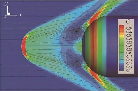
Fig.4 Time-averaged pressure contours and streamlines at axisymmetric plane and on body surface.
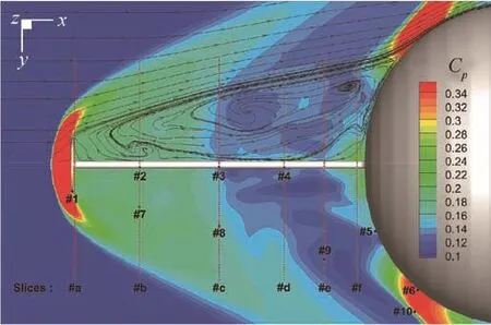
Fig.5 Instantaneous pressure contours and streamlines,with locations of pressure sample points and cross-sections.
To validate the flow solver,the test case by Gnemmi et al.14was selected with the in flow conditions as freestream Mach number Ma=4.5,Reynolds number ReD=5.0×10⁵,and temperature T∞=240 K.This study focuses on the cases at zero incidence.Moreover,the calorically perfect-gas assumption is adopted here.The corresponding experimental study of Gnemmi et al.14was conducted within the Institute of Saint-Louis(ISL)shock tube facility,on a model of a hemispherical shape of a diameter,D=0.07 m,representing the nose of a space vehicle.Fig.3 compares the computed and measured pressure coefficient Cpdistributions on the nose surface.It is seen that the grid independence is demonstrated and the present solver provides excellent agreement with the experimental data than that of Gnemmi et al.14Moreover,the pressure decrease in the spike-on case is almost 10 times the value obtained in the spike-off case,indicating that the drag reduction really benefits from the spike-disk combination.

Fig.6 Spectrum of pressure signals at Monitors#1 to#10.
Then,the investigation of the aerodynamic flow unsteadiness is conducted on the same model configuration with D of 2 m.The in flow conditions are set as Ma=3,ReD=2.72×10⁸and T∞=240 K.The time-averaged and instantaneous flow patterns are shown in Figs.4 and 5,respectively.It is seen that our flow solver accurately captures the features of flow around the model including the oblique foreshock,reattachment shock and shear layer.
Fig.5 depicts six pressure sample cross-section planes marked as#a to#f,and ten sample points marked as#1 to#10.The sample planes are located at xa=-0.895D,xb=-0.7D,xc=-0.45D,xd=-0.25D,xe=-0.125D and xf=-0.02D,while the points#1 to#6 are placed close to the body surface,#7 to#9 inside the shear layer and#10 nearby the reattachment shock.All monitors are set in the most pressure- fluctuation sensitive region,where there exists strong turbulence and/or shock/turbulence interaction.Note that the strongest turbulence appears at near-wall region and inside shear layer.
Fig.6 shows the power spectra amplitude of the pressure signals<p>at Monitors#1 to#10 as a function of the Strouhal number,St=f D/U∞.Note that the largest frequency is related to the sampling frequency f,which equals 1/Δt=100U∞/D,while the smallest frequency is determined by the total time of the sampling.As shown in Fig.7,the dominant amplitude in the frequency spectrum can be found at St1=0.092 for all monitors,and St2=0.004 in the shear layer(#1,#7 to#9).It is noted that the character frequency around 0.015(see Fig.7)is regarded as a harmonic one,partially due to its comparably small amplitude in all 4 spectra,partially due to the visible data scatter at 4 monitors(#2,#3,#6,#10).
Fig.8 reveals the flow pattern right upstream of the blunt nose,where there exists strong circumferential motion of the flow.This motion is due to the impingement of supersonic jets that are caused by fore-shock/bow-shock interaction,on the surface of the nose(see Fig.9(a)),as also observed in the experiment by Edney.23Fig.9(b)and(c)further show that such a strong circumferential motion occurs in the spike/nose junction region,where Monitor#4 is placed.As shown in Fig.6,a Strouhal number of 0.092,St1,is the peak frequency in the spectra analyses at#4,which implies that the ‘‘pulsation mode”6,7is characterized by St1.
Moreover,nearly perfect circular shape of mean- flow pattern can be obtained as the averaged time chosen as 20/St1,as shown in Fig.8(a).It indicates again that the dimensionless frequency of St1dominates in this region.If the mean- flow data is further circumferentially averaged,the Mach number distribution in the radial direction r/D(see Fig.10)shows that the most unsteady flow occurs inside the isoline of zero velocity magnitude(the red curves in Fig.8).
Figs.11 and 12 show that there appear 5 vortex rings right behind the aero-disk.Downstream of the 5th ring come out small turbulent structures.Fig.13 depicts the dynamic behavior of the vortex rings,in the time-dependent progression of their circumferentially averaged locations.It is seen that all the vortex rings are pretty stable.Note that Monitors#7 to#9 are placed in fore-shock/turbulence interaction region,and#7 locates very close to the 5th ring while#8 and#9 are surrounded by small turbulent structures.This explains why St2of 0.004 is the first peak in the spectra at Monitors#8 and#9,but the second peak at Monitor#7.Nevertheless,the‘‘oscillation mode”5has the characteristic frequency St2dominated by the fore-shock/turbulence interaction.And the step mode interacts with shedding mode in the reattachment region,resulting in the low-frequency characteristics.

Fig.7 Statistics of peak frequencies at all ten monitors.
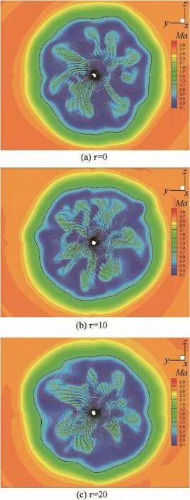
Fig.8 Instantaneous snapshots of velocity vectors and Mach number contours at#f plane.

Fig.9 Instantaneous flow using Q criterion at Q=-20 U∞2/D2.
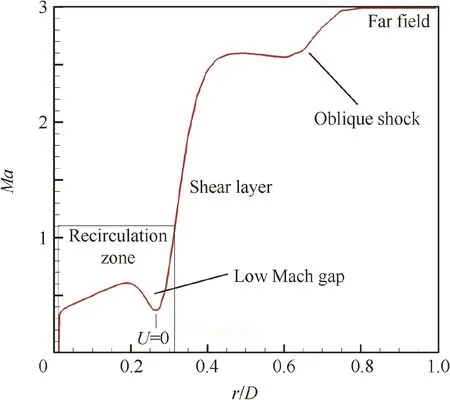
Fig.10 Time-and circumferentially averaged Mach number distribution in radial direction.
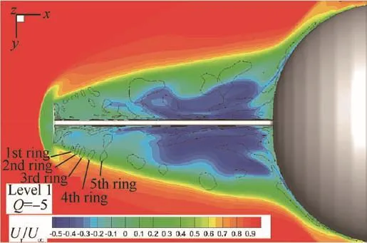
Fig.11 Axial velocity contours and isolines of Q=-5 U∞2/D2.

Fig.12 Instantaneous flow using Q criterion at Q=-5 U∞2/D2,shaded by dimensionless axial velocity Ua.

Fig.13 Time series of circumferentially averaged vortex-ring locations.
4.Conclusions
This paper has conducted a comprehensive numerical investigation of supersonic flows past a spike-tipped blunt nose.By using an in-house compressible flow solver,IDDES simulations were performed to resolve flow turbulence and shock structures.
The simulations well reproduced pressure coefficient on the entire body surface.The results show that there exist two distinct instability modes:oscillation mode and pulsation mode,with non-dimensional frequencies at 0.004 and 0.092,respectively.The foreshock/turbulence interaction results in the‘‘oscillation mode” that is characterized by a Strouhal number one order lower than the ‘‘pulsation mode” caused by the interaction between turbulence and shock structures around the blunt nose,as also observed in the measurement of unsteady spiked-body flows at Ma of 2.21 and ReDof 1.2×105.5,6The authors of this paper believe that with better understanding of unsteady features,effective control practice will be illustrated.
Acknowledgements
This work has been funded by the National Natural Science Foundation of China(Nos.11572177,11572176,51376106 and 11272183)and the Tsinghua University Initiative Scientific Research Program of China(No.2014z21020).
杂志排行

CHINESE JOURNAL OF AERONAUTICS的其它文章
- 80 years education of aerospace science and technology in Tsinghua University
- A brief overview of the School of Aerospace Engineering of Tsinghua University
- Subsonic impulsively starting flow at a high angle of attack with shock wave and vortex interaction
- High-order compact finite volume methods on unstructured grids with adaptive mesh refinement for solving inviscid and viscous flows
- Pressure distribution guided supercritical wing optimization
- A high- fidelity design methodology using LES-based simulation and POD-based emulation:A case study of swirl injectors