Super-resolution reconstruction of astronomical images using time-scale adaptive normalized convolution

Rui GUO ,Xioping SHI,Yi ZHU ,Ting YU

a Control and Simulation Center,Harbin Institute of Technology,Harbin 150080,China

b Tianjin Branch of China Petroleum Pipeline Engineering Company Limited,Tianjin 300457,China

KEYWORDS

Abstract In this work,we describe a new multiframe Super-Resolution(SR)framework based on time-scale adaptive Normalized Convolution(NC),and apply it to astronomical images.The method mainly uses the conceptual basis of NC where each neighborhood of a signal is expressed in terms of the corresponding subspace expanded by the chosen polynomial basis function.Instead of the conventional NC,the introduced spatially adaptive filtering kernel is utilized as the applicability function of shape-adaptive NC,which fits the local image structure information including shape and orientation.This makes it possible to obtain image patches with the same modality,which are collected for polynomial expansion to maximize the signal-to-noise ratio and suppress aliasing artifacts across lines and edges.The robust signal certainty takes the confidence value at each point into account before a local polynomial expansion to minimize the influence of outliers.Finally,the temporal scale applicability is considered to omit accurate motion estimation since it is easy to result in annoying registration errors in real astronomical applications.Excellent SR reconstruction capability of the time-scale adaptive NC is demonstrated through fundamental experiments on both synthetic images and real astronomical images when compared with other SR reconstruction methods.

1.Introduction

The engineering community that firstly encountered with image reconstruction and restoration was the space program in the 1950s.1The first sets of astronomical images captured from the Earth and the planets were of unimaginable resolution due to technical difficulties,such as diffraction blur,optical aberrations,noise,etc.These difficulties resulted in decimated, aliased extraterrestrial observations of an astronomical scene, and a multi-image-based Super-Resolution(SR)technique was introduced to retrieve as much additional information as possible from such degraded sequential astronomical images and reconstruct one High-Resolution(HR)astronomical image.Super-resolving observed Low-Resolution(LR)astronomical images has been proven to increase high-frequency components and remove degradations derived from ground-based optical astronomy imaging systems.There have been a considerable amount of image reconstruction and restoration techniques that achieve SR directing toward optical astronomy,especially since the discovery of the spherical aberration problem in the Hubble Space Telescope in 1990.2Molina et al.3provided a review of image restoration in astronomy and then proposed a Bayesian modeling and inference method to remove noise and blur in astronomical images.Starck et al.4described two novel multiscale approaches based on ridgelet and curvelet transforms instead of the wavelet transform,which present high directional sensitivity and can better show elongated details hidden in astronomical images.Wu and Barba5proposed an iterative optimization algorithm to restore star field images by using the minimum mean square error criteria and the maximum varimax criteria.

The classical multiframe SR reconstruction comprises three basic procedures:LR image acquisition,image registration,and HR image construction.Fig.1 describes a common image formation model concerned with an HR image to decimated,aliased observations with motion between a scene and a camera.From Fig.1,we can understand how LR observations are generated from detector limited imaging systems.The basic idea behind SR is that sampling diversity provided by the complementary information contained in multiple LR observations can be utilized to combat undersampling,making the ill-posed upsampling process better constrained.Therefore,SR reconstruction can be implemented by aligning LR images with subpixel shifts to reconstruct them on a new and greater image grid,achieving the inverse process of the observation model.

SR reconstruction was primarily presented by Tsai and Huang6in 1984,analyzing the basic characteristic of Fourier transform.Numerous novel SR reconstruction methods have emerged over the last two decades7,8,which can be divided into two main types,i.e.,spatial domain and frequency domain based methods.The formulation for SR reconstruction in Ref.6 assumed an idealistic observation model with known parameters,upon which many improvements have existed to deal with more complex situations.Kim et al.9developed Ref.6 by incorporating the motion blur and aliasing effect into a recursive procedure based on the weighted least square theory.They provided a further improvement in Ref.10 by introducing a recursive total least squares algorithm.Tom et al.11presented a new approach that solves restoration and motion estimation sub-problems simultaneously using the Expectation-Maximization (EM) algorithm. Frequency domain based methods have the merit of high calculation ef ficiency,but can only deal with limited image degradation models and restricted image priors from the reconstruction process.Later works on SR reconstruction have focused more on the spatial domain,providing its adaptability to handle different types of image observation models.Typical approaches include Iterative Back Projection(IBP),12maximum likelihood(ML),13Maximum A Posteriori(MAP),14and Projection Onto Convex Sets(POCS),15which improve the disadvantages of frequency domain based methods with more computationally intensive operations.

In the conventional multiframe SR reconstruction,image registration is critical for the performance of HR image reconstruction.A promising approach used recently is the nonparametric approach,which omits accurate motion estimation.Protter et al.16incorporated the denoising NonLocal-Means(NLM)algorithm with an accurate-motion-estimation-free property into SR reconstruction.Later,they further extended the NLM algorithm and proposed a probabilistic and crude motion estimation to achieve SR without a need for image registration in Ref.17Takeda et al.18presented an iterative 3-D framework for SR reconstruction by applying a 3-D steering kernel,19which is based on the local Taylor series of its spatiotemporal neighborhood,containing information about the local motion across time.However,the NLM algorithm can lead to produce noticeable aliasing,and the iterative 3-D framework based method requires multiple iterations and complex computations.

In this paper,we present a novel multiframe SR framework independent of accurate motion estimation,called time-scale adaptive normalized convolution,and apply it to astronomical images.The proposed SR algorithm is inspired from Normalized Convolution(NC)20where the polynomial basis function is utilized to express a weighted neighborhood of a target position for local signal modeling.Furthermore,signal certainty and spatially adaptive filtering are introduced to minimize the influence of outliers and adapt the underlying image structure,leading to robust and adaptive NC.Finally,temporal scale applicability is incorporated to the SR framework which aims to omit accurate motion estimation during SR reconstruction.

The structure of the paper is as follows.Section 2 reviews the concept of a robust and adaptive NC method along with its SR reconstruction results.Section 3 presents a time-scale adaptive NC method for SR reconstruction and its major advantages compared against other SR approaches.Experimental results are shown in Section 4,and Section 5 concludes.

2.Robust and adaptive normalized convolution

Normalized convolution is a method for each neighborhood of signal analysis onto a projective subspace which is expanded by basis functions.At the same time,this method takes uncertainties in signal values into account and enforces spatial localization of the signal model through an applicability function.Weights for the projection can be obtained by implementing a weighted least squares estimation,where a set of expansion coefficients at each signal point is achieved,one for each basis function.

2.1.Polynomial-based NC

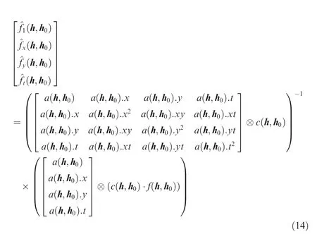
Many existing bases can be chosen,and the polynomial basis:［1，X，Y，X2，Y2，XY，...］is more commonly used in most applications, where 1= ［1，1，...，1］T(N samples), X=and so on represent the coordinates of N surrounding positions of the local signal.The application of polynomial basis functions allows the conventional NC to become a local Taylor series expansion around a central position at h0= ［x0，y0］,and the estimated pixel value at location h= ［x+x0，y+y0］can be expressed in terms of a polynomial expansion as follows:

where ［x，y］denote the corresponding coordinates of a certain position h around the central analysis pixel at h0.p（h0）= ［p0，p1，...，pm］T（h0）denotes a vector representing the expansion coefficients with respect to the polynomial basis functions at h0.For the polynomial order,we utilize the first-order NC for SR reconstruction,which can model enough edges at little computational cost.

Generally,NC implements the localization of the polynomial fit using an applicability function.A Gaussian function,which monotonically decreases in all directions with its isotropic property and flexible scale,is often used for this purpose.Besides,NC sets the certainty value for each input sample,given by non-negative real numbers,which is especially useful in the case of missing data outside the border of the signal.The applicability function and the signal certainty are two key factors to influence the result of expansion coefficients for each basis function.

2.2.Least-squares estimation

The projection coefficients p at position h0can be obtained by minimizing the approximation error ε（h0）according to the extension of an applicability function a（h，h0）around the central analysis pixel at h0as follows:

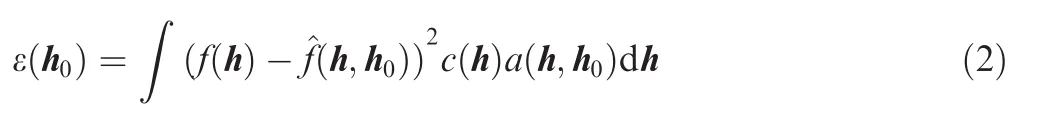
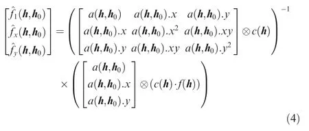
where c（h）denotes the signal certainty,which specifies the measure of confidence in the input samples at h,limited to the range of［0，1］.Both c（h）and a（h，h0）,considered as major factors for the approximation errors,increase the adaptability of the image structural content as described below.For each analysis window containing N samples,the projection is equivalent to a weighted least squares problem,resulting in a matrix representation21as follows:

where B= ［b1，b2，...，bm］denotes an N × m matrix with respect to m basis functions based on N surrounding positions,f denotes an N×1 matrix of the local image content,and W=diag（c（h））.diag（a（h，h0））denotes an N × N diagonal matrix derived from a pointwise product result of the signal certainty c（h）and the applicability function a（h，h0）.

The full first-order NC is given by

2.3.Robust NC

Polynomial expansion and applicability functions unfortunately are,in most cases,assumed to perform at irregular local coordinates.As a useful approach to deal with irregularly positioned uncertain data,NC allows the certainty value to be established before processing.A Gaussian function based on the estimated differencewhich uses a weighting scheme based on geometric closeness and photometric similarity proposed in bilateral filtering,22is chosen as the robust certainty in NC.The robust certainty is designed to remove potential outliers from the analysis in the neighborhood around h0before implementing local polynomial expansion,which is defined as

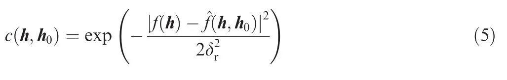
where f（h）denotes the pixel value of the observed image at position h,and）denotes the estimated pixel value at h which is approximated by the polynomial basis function with respect to the central analysis pixel at h0.The robust certainty function c（h，h0）is somewhat preferable to the fixed certainty c（h）in Eq.(2)because c（h，h0）can change along with the movement of the window of analysis rather than depending only on the global coordination h.The photometric spread σris designed to provide a reasonable range for the estimated differencewhich is twice the intensity value of the observed noise σnoise.As a result,all samples with an estimated difference in the range of±2σnoisedeviations get a certainty value close to one.

2.4.Shape-adaptive NC

In astronomical applications,captured images are insufficient,and an applicability function with linear structures cannot preserve image details,such as lines and edges.A shape-adaptive applicability function is introduced to significantly improve the quality of sparsely sampled data convolution,where an anisotropic Gaussian kernel is used along the underlying image structure,providing a better denoising effect and guaranteeing the continuity of the structural content across lines and edges.The chosen applicability function adapts the kernel’s shape and orientation,making it possible to obtain samples with a similar output intensity and image gradient.These samples are collected for polynomial expansion which is available for NC of any order.

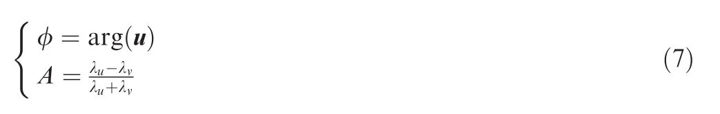
To obtain an adaptive kernel for each output pixel,the underlying structural content around each position must be confirmed before processing.Firstly,a preliminary estimation of the interpolated image I and gradient images in two directions Ix= ∂I/∂x and Iy= ∂I/∂y is calculated through the first-order robust NC in Eq.(4).This calculation is then applied to the Gradient Structure Tensor(GST)method,23given by

where ［λu，λv］（λu≥ λv）denote the eigenvalues derived from the local gradient vectors ▽I= ［Ix，Iy］T,and ［u，v］denote the associated eigenvectors.The orientation φ and the anisotropy A,which are considered as the local image structure information,can be obtained using the GST method,given by

Local sample density also needs to be taken into account as an important data parameter,which represents how much information is valid around the surrounding points.In most cases,the sample density of uncertain data can be obtained by calculating the sum of the certainty of all regular grid samples based on the local scale component as follows:

where σc（h0）denotes the local scale with respect to an unnormalized Gaussian weighted function,and d（h0，σc）is defined as a constant 3 for first-order NC.This scale is then employed to shrink or grow the applicability function and reduce unnecessary smoothing associated with a high local sample density.

Finally,an anisotropic Gaussian function serves as the adaptive applicability function in this subsection,which is mathematically represented as

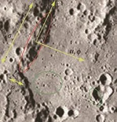
Fig.2 An example of shape-adaptive applicability functions in an astronomical image.

where h0= ［x0，y0］denotes the central analysis pixel,and h-h0= ［x，y］denote the local coordinates of surrounding positions around h0.γ denotes a pillbox function ensuring the kernel matrix within a fixed radius.σuand σvdenote two local adaptive scales of the anisotropic Gaussian kernel in each dimension,and can be changed adaptively depending on the estimated local scale σc（h0）,which is given by

The difference between the two directional scales is that σvrepresents the scale which is elongated in one direction and greater than or equal to σu(described in Fig.2).Furthermore,parameter κ is set to a constant 0.5,which is considered as the upper limit of the range of the applicability function to keep the anisotropic Gaussian kernel from degenerating to a distorted ellipse function.

2.5.Robust and adaptive NC for SR reconstruction

The sections above follow an SR approach with three steps called robust and adaptive NC method as depicted in Fig.3.Firstly,multiple LR observations are registered relative to a uniform grid with subpixel precision utilizing an efficient subpixel image registration algorithm.24Next,robust and adaptive fusion is then implemented on these registered LR observations utilizing the robust and adaptive NC method.Finally,deconvolution25can achieve a better deblurring and denoising effect.The whole SR process in Fig.3 is further subdivided into three separate steps,gradually enhancing the resolution of HR image reconstruction.The initial estimate HR0is obtained using bicubic interpolation,which is then applied to first-order robust NC to further improve the reconstruction result of the HR image HR1and its gradient information HRxand HRy.The gradient information is then utilized to form the anisotropic applicability function for implementing the final robust and adaptive NC.

3.Time-scale adaptive NC for SR reconstruction

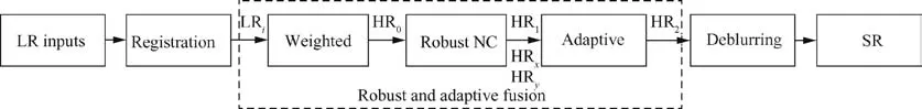
Fig.3 Robust and adaptive NC for SR reconstruction.

Before we apply robust and adaptive NC to the SR framework,accurate image registration is required for the recovery of sub-pixel details.However,a highly accurate motion estimation is extremely hard to achieve,especially in ground-based optical astronomy imaging systems,easily resulting in registration errors and limiting the reconstruction result.Therefore,to avoid this problem,all observations in the LR image sequence can be considered as a whole ‘‘image” with an additional temporal scale,where robust and adaptive NC is improved to time-scale adaptive NC for SR reconstruction.Different from robust and adaptive NC,whose applicability function at position h0is dependent on all the registered surrounding samples,forming the shape of an oval contour,the contour of the applicability functions in time-scale adaptive NC can be defined as an ellipsoidal shape centered at h0（h0= ［x，y，t］）.The ellipsoid surface formed in the local image structure introduces temporal scale applicability which makes HR image reconstruction without a registration process become possible.

3.1.Time-scale adaptive NC

Time-scale adaptive NC is obtained by an improvement of robust and adaptive NC,and the polynomial basis is extended to ［1，X，Y，T，X2，Y2，T2，XY，XT，YT，...］,where T denotes the local coordinate based on the temporal scale.The estimated value at location h= ［x+x0，y+y0，t+t0］is expressed as a local Taylor series expansion by the following extended polynomial basis:

where ［x，y，t］denote the local coordinate of a certain position h in the additional temporal scale around h0.denotes a vector representing the expansion coefficients with respect to the extended polynomial basis functions at h0,and m denotes the size of the basis functions.Within a local image structure,p0represents the estimated intensity,while p1,p2,and p3represent the corresponding gradient information.

The projection coefficients pts（h0）can be obtained after the applicability and certainty functions are established.Based on the above discussion,a standard least-squares solution is applied to minimize the following approximation error in time-scale extension:

The analysis window in Eq.(12)is changed to be within a cube instead of a plane in Eq.(2),and the result of leastsquares estimation in a matrix form can be expressed as

The full first-order time-scale NC is implemented which can be expressed as

To solve the problem of its computational complexity due to the correlation between each frame,cts（h，h0）is just ensured by those frames where h and h0are in the same temporal dimension,i.e.,the certainty function in a frame is irrelevant to the one in other frames.The simplified form of the certainty function is given by

We assume that the coordinate of h0is（x，y，t）,and the certainty function in Eq.(15)is just obtained from a fixed frame instead of being achieved through all the neighbor samples around a fixed position,thereby simplifying the amount of calculation.

The shape-adaptive applicability function in the time-scale adaptive NC is also improved in this section.Firstly,we calculate a preliminary estimation of the interpolated image I and gradient images Ix,Iy,and Itutilizing the first-order timescale NC in Eq.(14).Then,the gradient structure tensor can be obtained by

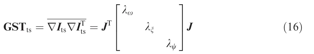
where ▽Its= ［Ix，Iy，It］Tdenotes the local time-scale gradient vector with respect to GSTts.J denotes a transform matrix in the form of diagonal orthogonal decomposition based on GSTtsinvolving all three orthogonal eigenvectors,and λω,λξ,and λψdenote the three eigenvalues.

Next,the local orientation and scale can be determined based on the above decomposition form.In the time-scale adaptive NC,a novel orthogonal coordinate system is introduced including three directions,instead of judging which the elongated direction is and deducing its orthogonal direction in robust and adaptive NC.The projection values corresponding to the three orientations are given as

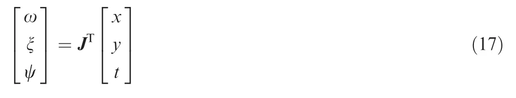
where ω,ξ,and ψ denote the projection values from three new directions,which are transformed from the local coordinate in the x-y-t coordinate system.These projection values can be used to establish the local features of the applicability function.

An anisotropic Gaussian kernel is still treated as a shapeadaptive applicability function in the time-scale adaptive NC.Local structures can be identified by these three different eigenvalues.We assume that the eigenvalues are in the form of a descending order by λω＞ λξ＞ λψ,and different local structures can be obtained by

(1)If λω≈ λξ≈ λψ≈ 0,the local image structure is equivalent to a flat area.

(2)If λω≈ λξ≈ λψ＞ 0,the local image structure is equivalent to an isotropic area or an angular area.

(3)If λω＞ λξ≈ λψ≈ 0,the local image structure is equivalent to a layered texture area or borders.

(4)If λω≈ λξ＞ λψ≈ 0,the local image structure is equivalent to an edge or corner area.

Besides,three variables are defined to estimate the local scales,which is given by

The three variables are limited to the range of［0，1］,and the local scales in the time-scale adaptive NC are represented as

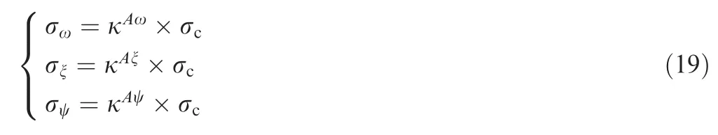
where κ is utilized to control the change ratio of scales which is set to 20 in this section,and σcdenotes the local sample density parameter.The robustness of scales can be enhanced due to the fixed scopes of Aω,Aξ,and Aψ.

The local sample density σc（h0）in the time-scale adaptive NC can be estimated by

where dts（h0，σc）is set to a constant 4 in order to ensure that the sampling of input images is enough.To obtain this local scale,an estimation algorithm is utilized in this subsection as shown in Fig.4.Firstly,the certainty value for every input sample is divided into its four closest coordinates on the HR image grid using the bilinear-weighting method.Next,a density image is mapped onto the HR image grid by collecting all grid-marked sample certainty values,whose Gaussian scale space can be formed utilizing a recursive algorithm for the Gabor filter.26The filter weights for the Gabor kernel are unnormalized,and the scale spatial responses corresponding to each sample increase with a second-order rate.Finally,we can implement a bilinear interpolation on the HR image grid along the scale axial direction to achieve the Gaussian scale when its scale spatial response is equal to an appropriate constant.

Finally,the time-scale applicability function can be represented as

where f（h）and f（h0）denote the intensity values at h and h0,respectively.u（h0）,v（h0）,and w（h0）denote the projection values,and σu（h0）, σv（h0）,and σw（h0）denote the directional scales.Besides,γtsis defined as a function,which is given by

where σγis set to 6 to balance the proportion between the image smoothness and sharpness when a proper value of this parameter is considered.The effect on the applicability function based on σγmakes γtsassign the photometric weights according to the intensity difference f（h）-f（h0）.Moreover,exp（·）in Eq.(21)corresponds to the spatial weights and temporal scale applicability.

3.2.Time-scale adaptive NC for SR reconstruction

Fig.4 Fast estimation algorithm of the local sample density.

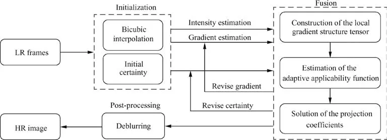
Fig.5 Time-scale adaptive NC for SR reconstruction.

Fig.5 presents the improvement algorithm of time-scale adaptive NC for SR reconstruction in this section,which follows three separate steps.The preliminary certainty function for each position is firstly established through robust and adaptive NC,and bicubic interpolation for all LR observations is performed to obtain the preliminary estimates of the intensity and gradient values for the HR image.In the following fusion step,the preliminary estimates are utilized to further revise themselves,as well as the certainty function.In order to achieve more accurate SR reconstruction,the gradient value is calculated by applying the time-scale adaptive NC to the reconstruction process and deriving from the projection coef ficients.Three iterations are implemented in this algorithm where the results of the previous iterative computation are considered as the inputs in the next iterative computation.As a final step,a deconvolution algorithm is applied to remove the blur and noise elements to produce the final reconstruction image.The detailed procedures of the improved SR reconstruction method are presented in Table 1.

The improved time-scale adaptive NC has three major superiorities compared against other SR approaches:(A)the directional scales in the time-scale adaptive NC can be adjusted to suit different local structures which can be seenas the self-adapting filter.Therefore,the process of fusion and denoising can be accomplished simultaneously in the second step;(B)the SR reconstruction process does not require an accurate motion estimation;(C)the local structure for each point is constructed using the gradient information in the GST instead of its neighborhood pixels.Thus,less computational time is required in this condition.In addition,the certainty function existing in the improved time-scale adaptive NC also provides robustness to potential outliers.

Table 1 Summary of the time-scale adaptive NC for SR reconstruction.

4.Experiments

In this section,a number of SR experiments are carried out on simulated data and real astronomical images where we compare the performance of the time-scale adaptive NC method with those of several other benchmark techniques in terms of HR image restoration quality.

4.1.SR results on simulated data

The simulated data consists of four HR images with a size of 256×256,as shown in Fig.6,which are used to generate four synthetic image sequences,each including six LR images.To simulate the real imaging system,the four HR images are warped,blurred,and downsampled by a decimation factor of 2:1.We consider a motion model sk= ［θk，ck，dk］Tcontaining translational and rotational information,where θkdenotes the rotation angle,and ckand dkdenote the translations of the k th LR observation relative to the reference image in horizontal and vertical directions,respectively.The following motion vectors:s1= ［0.0°，0.0，0.0］T,s2= ［0.0°，0.5，0.5］T,s3= ［1.0°，0.0，0.5］T,s4= ［-1.0°，0.5，0.0］T,s5=［3.0°，1.0，0.0］T,and s6= ［-3.0°，0.0，1.0］Tare chosen for the images in the sequences.For blurring,we use a 3×3 uniform Point Spread Function(PSF).Finally,the LR observations are further contaminated by an additive white Gaussian noise at different Signal-to-Noise Ratio(SNR)levels of 5,15,25,35,and 45 d B.Simulation experiments based on 10 different noise realizations with respect to different SNR levels are implemented,and we record the mean values of these experiments.Besides,a 20×20×5 local analysis window is incorporated in the high-resolution grid and a 3×3 Gaussian PSF with std=1.5 is applied for deblurring.Note that just the pixels derived from the initial LR observations are used to construct the underlying image structure,not all the pixels derived from the local analysis window.

Fig.6 Set of 256×256 images processed in synthetic experiments.

For comparison,the following SR reconstruction techniques are utilized:(A)bicubic interpolation(denoted by BCB),(B)the non-local means in Ref.16(denoted by NLM),which is combined with a local and patch-based approach,(C)the 3-D ISKR in Ref.18,which is based on multidimensional kernel regression,and(D)the robust and adaptive NC in Section 2.

To measure the quality of the reconstructed HR images acquired using these different techniques quantitatively in synthetic experiments,the Peak Signal-to-Noise Ratio(PSNR)is used,which is expressed as

The mean PSNR values derived from all these SR reconstruction techniques mentioned above,for the four images in Fig.6(a)–(d)with all SNR levels,are plotted in Fig.7(a)–(d).As expected,all SR reconstruction techniques perform better according to the PSNR value than BCB.It is evident that the time-scale adaptive NC algorithm(3 times iterations)shows the maximized performance on the recovery of HR images by utilizing all SR reconstruction techniques with all SNR levels,which offers slightly higher PSNR values than those of robust and adaptive NC.It should be emphasized that the PSNR value in the first iteration of the time-scale adaptive NC algorithm is slightly higher than those derived from the second and third iterations,where the estimation error of the underlying image structure becomes the biggest restrictive factor.Moreover,a smaller regularization parameter is adopted to remove the blurred components in the time-scale adaptive NC algorithm which can produce sharper edges with less ringing artifacts but bring lower PSNR values.Another important thing to note is that the BCB method and robust and adaptive NC need to use registration algorithms,while the rest experimental methods omit accurate motion estimation.

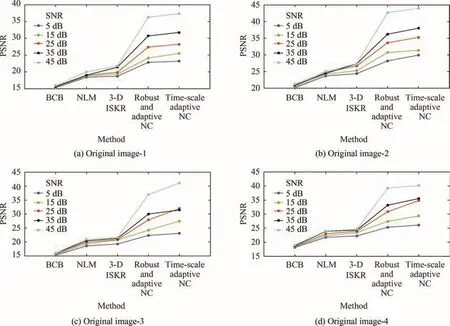
Fig.7 Mean PSNR values for the images in Fig.6(a)–(d).

To better show the SR reconstruction performance of the time-scale adaptive NC algorithm,we provide sixteenth-times SR for a Region Of Interest(ROI)which contains more details and is useful for vision observation.The reconstruction images are presented in Fig.8,where the LR images and the results of BCB,NLM,3-D ISKR,robust and adaptive NC,and timescale adaptive NC(one time iteration),for the images in Fig.6(a)–(d)when SNR=25 dB,are arranged from the first row to the sixth row.

As can be seen in Fig.8,the results obtained by BCB significantly reduce aliasing artifacts and improve the clarity of many small features,where the process relies on very exact motion estimation for the recovery of sub-pixel details,but still cause serious jaggy artifacts along edges and cannot remove noises and outliers efficiently.The NLM method is designed to denoise image sequences without accurate motion estimation where minimization of an energy function leads to a powerful and effective denoising algorithm.The results from this method remove low noises but not strong outliers,and still seem crisp and somewhat over-sharpened.For the 3-D ISKR algorithm,the space-time(3-D)steering kernel regression makes the pixels in a local neighborhood equivalent to an iterative 3-D framework,which can obtain the spatial and temporal behaviors of its local image structures and contain accurate motion information.The results improve the overall performance,but encourage unwanted annoying noisy artifacts in flat areas.By contrast,the results from robust and adaptive NC and time-scale adaptive NC achieve the best reconstruction results with considerably fewer noisy artifacts and much sharper edges than those of the other SR reconstruction techniques,which is particularly obvious in high-noise situations.The difference between them is that the HR images restored by time-scale adaptive NC provide slightly higher quality than that by robust and adaptive NC and require no accurate motion estimation.

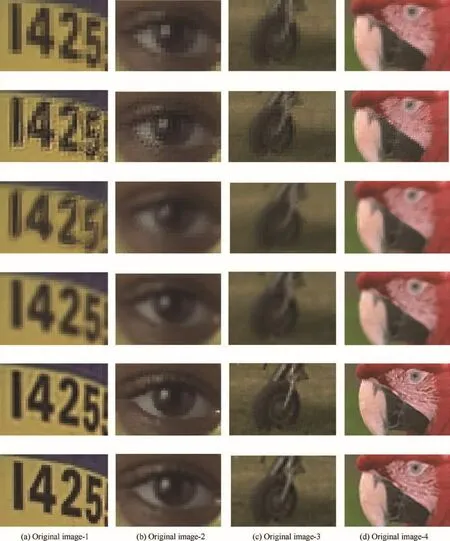
Fig.8 Sixteenth-times SR results for the images in Fig.6(a)–(d)when SNR=25 dB.

4.2.SR results on real astronomical images

Next,we show example SR results with two real astronomical image datasets,where 20 sequential LR images of the lunar surface were taken from a Canon EOS 70D camera and a TW-CMV20K camera through an astronomical telescope(see Fig.9),respectively.We utilize the same methods as in the experiments on simulated data for demonstrating the performance of the time-scale adaptive NC and increase their resolution by a factor of P=2.Figs.10 and 11 show the sixteen-times SR results obtained by BCB,NLM,3-D ISKR,robust and adaptive NC and time-scale adaptive NC(one time iteration),for the images in Fig.9(a)and(b),respectively.The results from BCB show jaggy details and blurring artifacts along crater edges on the lunar surface.The results from the NLM method and the 3-D ISKR method further preserve sharp image features along lunar crater edges and suppress noise and serious jaggy artifacts.The superior quality of the SR reconstructions obtained by robust and adaptive NC and time-scale adaptive NC is evident,providing a high level of details without blurring and noise which is particularly obvious around the details on the lunar surface in both images.Robust and adaptive NC and time-scale adaptive NC generate very similar results,but the ringing artifacts around lunar crater edges in time-scale adaptive NC results are more suppressed than those of robust and adaptive NC.

Fig.9 Set of real astronomical images taken from a Canon EOS 70D camera and a TW-CMV20K camera.

Fig.10 Sixteen-times SR reconstruction for the image in Fig.9(a).

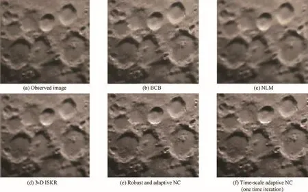
Fig.11 Sixteen-times SR reconstruction for the image in Fig.9(b).

5.Conclusions

We present a novel SR framework for astronomical images using time-scale adaptive NC which is combined with the conceptual basis of conventional normalized convolution.A robust polynomial expansion is utilized to express an adaptive neighborhood of each position for local signal modeling,and polynomial coefficients can be obtained by implementing weighted least squares fitting.The introduced shape-adaptive applicability function detects and enhances local linear or edge structures to collect more image patches with the same modality for a better analysis.The robust sample certainty is automatically attached with each position according to the intensity difference against the center of analysis,effectively excluding potential outliers from the local analysis window.However,there exist decimated and aliased elements caused by incomplete image information in real astronomical applications,because it is difficult to achieve accurate sub-pixel motion estimation.In order to solve this problem,temporal scale applicability is considered to form improved time-scale adaptive NC.

An experimental evaluation of the effectiveness of the timescale adaptive NC has been made on simulated data and real astronomical images.In SR results,the time-scale adaptive NC outperforms other discussed SR reconstruction techniques such as bicubic interpolation,the NLM algorithm,and 3-D ISKR,and obtains reconstruction results with slightly better performance than those of robust and adaptive NC.Furthermore,the time-scale adaptive NC is also robust against decimated and aliased elements and requires no accurate motion estimation.

Not only useful in multiframe SR reconstruction,time-scale adaptive NC can also deal with several applications such as orientation estimation,displacement estimation,analysis of interlaced signals,and video SR reconstruction.