Development of secondary flow field under rotating condition in a straight channel with square cross-section

Ruquan YOU ,Kuan WEI,Zhi TAO ,Haiwang LI,*,Guoqiang XU

a National Key Laboratory of Science and Technology on Aero-Engines Aero-Thermodynamics,Beihang University,Beijing 100083,China

b Collaborative Innovation Center for Advanced Aero-Engine,Beihang University,Beijing 100083,China

c Aero Engine Academy of China,Aero Engine(Group)Corporation of China,Beijing 101304,China

KEYWORDS

Abstract The developing secondary flow fields in the entrance section of a rotating straight channel were experimentally investigated using Particle Image Velocimetry(PIV).The effects of streamwise position,Reynolds number and rotation number on the development of the secondary flow fields were revealed.The results show that the absolute values of vorticity flux of the trailing side roll cells increase with increasing radius of the measured plane and rotation number.When the absolute value of vorticity flux exceeds a critical value,the merging of the trailing side roll cells appears.Moreover,when the number of the trailing side vortex pairs is even,the absolute values of vorticity flux of the leading side vortices increase along streamwise direction.Otherwise,the absolute values decrease along the streamwise direction.By the circulation analysis,this phenomenon was found to have relationship with the merging of the trailing side roll cells,and further concluded that the secondary flow field in a rotating channel has to be treated as a whole.At last,the increase of the Reynolds number was found to be able to induce the merging position moves upstream.

1.Introduction

To improve the thermal efficiency of modern gas turbine engine,the turbine blade has to be operated in the environments with extremely high temperature(＞1900 K)which is far beyond the suitable working temperature,even the melting point of the turbine blade material.To resolve this conflict,lots of cooling techniques were applied to protect the turbine blade.Internal cooling technique is one of the most classical and popular methods used to protect the turbine blade.As an effective method,serpentine passage in the middle section of a turbine blade was developed.1,2Most of the previous work was focused on the heat transfer in the serpentine passages because the heat transfer is the intuitive phenomenon and is easier to be measured than the flow field.However,sometimes the heat transfer phenomenon was not able to be explained reasonably because of a lack of the knowledge about the flow behavior under rotating condition.In order to enrich the knowledge in this field,some previous work focused on the primary flow fieldsin rotating channels.In these work,a variety of experimental techniques were utilized.For instance,Bons and Kerrebrock3measured the velocity profiles of the primary flow in a square cross-section rotating channel with PIV;Macfarlane and Joubert4investigated the developing boundary layersin threerotating channelswith different aspect ratio using hot wire.The current work also investigated the flow fields in a rotating channel.However not the primary flow fields,the secondary flow fields are the main concern of the present work.

Nomenclature

Why the secondary flow fields?Because the secondary flow fields deeply affect the primary flow and the heat transfer in the rotation channel.4Macfarlane et al.5defined the secondary flow strength and claimed that if this secondary flow strength exceeded a critical number,the secondary flow would influence the boundary layer development in a rotating channel.

The history of studies on the secondary flow field in a rotating channel can be stretched back to 1971.Lian et al.6investigated the stability of the secondary flow vortex structures in a rotating channel with AR=8:1.15 by both the flow visualization experiment and the theoretical analysis,where AR means aspect ratio.The experimental results demonstrated the existence of three secondary flow regimes in a rotating channel.That is,when the rotation number is smaller than a critical value,there was only a slightly straightening of the dye lines in the boundary layer.On the contrary,when the rotation number is larger than this critical value,a waviness of the dye lines was observed.If the rotation number increased further and the flow passed into the Taylor-Proudman regime,the most essential characteristic of the Taylor-Proudman regime flow was detected,the dye lines in the core region were parallel to the axial direction.Furthermore,Lian et al.6carried out a linear stability analysis about the onset of the waviness for the dye lines,namely the roll cells instability.Lezius and Johnston7also conducted a linear stability analysis about the instability of the onset for the roll cells.

Speziale and Thangam8numerically studied the same problem with Lian et al.6,and gave some secondary flow streamlines in detail.The results show that,for a given Reynolds number,when the rotation number Ro was smaller than a critical value,there is a symmetric vortex couple in the cross section plane.Meanwhile,when the rotation number is larger than this critical value,a series of small vortices appear near the trailing side.As the rotation number increased furthermore and exceeded another critical value,the flow passed into the Taylor-Proudman type regime.In this regime,the small scale vortices disappear,and the symmetric vortex couple reappeared.Moreover,the stability boundary for the appearance of small vortices was obtained.

Speziale9repeated Lian’s6experiments but changed the aspect ratio of the channel from 8:1.15 to 2:1.The similar transition process of the secondary flow revealed by Lian et al.6was also discovered by Speziale.

Besides the three stages,some other complicated transition phenomena were also found in the secondary flow transition process.

Smirnov and Yurkin10conducted a flow visualization experiment in a rotating channel with the aspect ratio equaling to 1.The experiments were carried out with water,and the flows were visualized by hydrogen bubbles and dye lines.By analyzing the results,nine flow regime boundaries were discovered;there was the stability boundary for the onset of the small vortices near the trailing side among them.

Kheshgi and Scriven11numerically studied fully developed laminar flow in a rotating channel with the aspect ratio equaling to 1.The three stages of the secondary flow transition process were also discovered.It is notable that an analysis of the secondary flow transition process from the intermediate rotation number regime to the high rotation number regime was given.In the phase chart,the four-vortex solution branch was found to be connected with the two-vortex solution branch by a pair of turning points.At the same time,the flow fields indicated that there is an unstable solution branch between this pair of turning point,which is to say,the transition process from the four-vortex solution branch to the twovortex solution branch is unstable.

Nandakumar et al.12carried out a research on the same problem with Kheshgi and Scriven.11With the decreasing of the rotation number from infinite to 0.2,many new solution bifurcations were found.It means that for a given rotation number there are variable possible solutions,some of which are two-vortex solutions,and the others are four-vortex solutions.In addition,the effects of secondary vortex structure on the primary flow was also shown in this paper.The fourvortex solution was found to be able to induce a defect of streamwise velocity near the trailing side.

It is worth mentioning that all the work above were conducted with laminar flow.

For turbulent flow,Watmuff et al.13measured the secondary flow near the trailing side in a rotating channel with the aspect ratio equaling to 4:1 using an X-type hot wire.In this work,the Reynolds number ranged from 119175 to 238351,and the rotation number ranged from 0.1 to 0.2.The results showed that there were a series of small vortices near the trailing side.Furthermore,these small vortices induced a wavy distribution of the skin shear stress along the spanwise direction on the trailing side.

Iacovides and Launder14numerically studied fully developed turbulent flow and heat transfer in rotating channels with aspect ratio equaling to 1:1 and 2:1,respectively.It was found that the Nusselt number on trailing side first increased with rotation number,then the increase ceased,and a Nusselt number plateau appeared,two small vortices were found near the trailing side.So,the appearance of the Nusselt number plateau was attributed to the small vortices.

Pallares and Davidson15conducted a Large Eddy Simulation(LES)research on the fully developed rotating channel flow.The variations of the secondary flow in the rotating channel from low rotation rate to high rotation rate were given.

Apart from the work on the secondary flow in a straight channel with rectangular cross-section,there are some investigations on the secondary flow in the U turn of a rotating channel or in a non-rectangular cross-section rotating channel.

Elfert et al.16measured the secondary flow in a rotating channel with U turn using non-rotating PIV system.However,they did not obtain the vortex structures in the straight section and only gave the secondary flow in the U turn section.That is because there is much higher accuracy of the secondary flow velocity in the U turn section than that in the straight section,since the secondary flow velocity in the U turn section is much larger than that in the straight section.Subsequently,Elfert et al.17extended the secondary flow research to the straight section with an engine-similar layout.To reduce the error introduced by the variation of the rotating speed,an improved sequencer technique was developed.

Gallo et al.18,19measured the secondary flow in the U turn section of a two-pass rotating channel with PIV,and reconstructed the 3D flow field in the U turn section.Liou et al.20–23measured the secondary flow in the U turn section of a twopass rotating channel with Laser Doppler Velocimetry(LDV).

In a word,the secondary flow in a rotating channel has attracted much attention in the past decades.However,most of the numerical researches focused on fully developed flow.For experimental researches,it is very hard to constitute a fully developed flow in a rotating channel,so all the experiments were conducted in developing flows,including the present work.However,unlike the present work,where most of these experimental studies were conducted in a rotating two-pass square channel or in a rotating channel whose cross section is not square.Special experimental research for the development of the secondary flow in the rotating single-pass channel with rectangular cross section is still rare in the open literature.To the best knowledge of the authors,only the group at The University of Melbourne implemented some experiments to study this issue using X-type hot wire.5,13However,there are two disadvantages to study the secondary flow fields using hot wire: first,measuring a three dimensional flow using an X-type hot wire probe is inappropriate because the measurement is liable to be interfered by the velocity component of the primary flow;second,it’s very hard to obtain the variations of the secondary flow under different conditions,because the hot wire probe can only measure the velocity point by point.

The aim of the present work is to fill this blank and study the variations of the secondary flow under different conditions in the rotating single-pass channel with rectangular cross section.The PIV technique was utilized.Limited by the accuracy and spatial resolution of the measurements,only the morphological study of the secondary flow fields was done.The measurements were conducted at three streamwise stations(x/d=5.5625,6.5625 and 7.5625)to study the streamwise development of the secondary flow with Reynolds number(Re=Umd/ν)ranging from 4750 to 9500 and rotation number(Ro=Ωd/Um)ranging from 0.125 to 0.75.It is notable that as the experiments were conducted in the entrance section of the channel,the boundary layers were still developing.In addition,although the Reynolds number based on the bulk mean velocity and the hydraulic diameter of the channel ranges from 4750 to 9500,the boundary layer flow under stationary condition were still laminar flow,because the turbulence intensities of the core region flows damped to about 1%with the help of the very fine screens.24

2.Apparatus and techniques

2.1.Rotating facility and test section

Fig.1 Rotating test facility.

Fig.1 shows the general arrangement of the rotating test rig,which consists of a disk rotating around a vertical shaft,and a 720 mm long test section.The rotating test rig is driven by a DC motor whose rotating speed is controlled by a digital converter(Eurotherm SSD 590).In addition,a high accuracy encoder(Renishaw Tonic T2000)is installed on the shaft as shown in Fig.2 to provide the accurate angle value for various applications,such as rotating speed measurement.Further details will be introduced below.

Air provided by a blower(RHG-520)was first mixed with the seeding particles to ensure that the seeding particles are uniformly distributed in the test section,and then the air passed through a float type flow meter before entering the rotating test rig through a rotary joint.In the present work,DEHS(Di-Ethyl-Hexyl-Sebacat)droplets(＜1 μm)generated by a Laskin-nozzle-based seeding particle generator were used as the seeding particles.Before entering the test section,the seeded air passed through a settle section,ensuring that the flow was approximately irrotational relative to the rotating channel at the entry of the test section.The settle section includes an expansion section,a honeycomb section and a screen section.

Fig.3 shows the isometric sketch of the test section,which defines the coordinate system,the trailing and leading walls for the given rotation direction,and an array of the test planes.The test section,720 mm in length,has a 80 mm×80 mm cross-section,with the entrance of the test section 211 mm away from the center of shaft.The secondary flow fields were measured respectively in the planes with x=445,525,605 mm,which are denoted by Plane 1 to Plane 3.

2.2.PIV technique

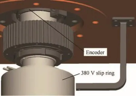
Fig.2 Encoder.

Fig.3 Test section.

The PIV is an optical measurement technique,which enables the simultaneous acquisition of velocity data over an area illuminated by a laser light sheet.17In the present work,the light pulses were generated by a dual-cavity 135 mJ Nd:YAG pulse laser device(532 nm)and guided via a light-guide arm to the desired test plane with a thickness of about 1 mm,and the digital imaging device was a Charge Coupled Device(CCD)camera (2048 pixel×2048 pixel,14 bits,14.7 frame/s)with a macro lens(105 mm).The measurements were conducted on Plane 1,Plane 2 and Plane 3,as shown in Fig.3.Table 1 lists the experimental parameters used for PIV acquisition on different planes.To make sure the mean secondary flow fields were statistically converged,500 image pairs were captured for each case.Fig.4 shows the convergence process of the velocity profiles obtained in a line on Plane 2 where z=40 mm and y=0–80 mm.Five different image pair numbers were tried to test the convergence of the results.It is obvious that 500 image pairs are enough to ensure the convergence of the results.

The collected image pairs were analyzed using the software Flow Master,and a flow field was calculated using the twopasses PIV interrogation algorithm.In the first pass,the dimensions of the sampling interrogation region were 64 pixel×64 pixel with half overlap,and then changed to 32 pixel×32 pixel with half overlap in the second pass.

In order to increase the accuracy of the secondary flow field,the particle displacement induced by the secondary flow between the first image frame and the second image frame has to be as large as possible.However,this displacement was restricted by the time that a seeding particle could stay in the laser light sheet.

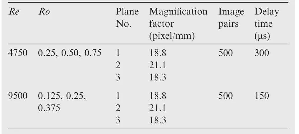
Table 1 Experimental parameters used for PIV acquisition.

Fig.4 Convergence process of velocity profile obtained in a line on Plane 2(z=40 mm,y=0–80 mm,Re=4750,Ro=0.25).

To increase the time that a seeding particle could stay in the laser light sheet,the second laser light sheet was purposely adjusted not overlapped but a little downstream to the first one,and the misalignment between them was about 0.3 mm.This is realized by adjusting the mirrors before the second harmonic generator to make the combination of two laser beams worse.The adjustable range is very small,otherwise,the second laser light sheet will be too thick to be used.

To balance the displacement of the seeding particle in the test plane and the error induced by the out-of-plane loss of correlation,the delay time was chosen to allow the seeding particles to move about 0.3 mm along the streamwise direction.

Once a vector field has been calculated,the vector validation algorithm can be applied to eliminate spurious vectors.In the present work,the peak ratio value was used as a postprocessing criterion for eliminating questionable vectors below a ratio-threshold,which was set to be 2.After the validation procedure,almost 15%of the vectors were rejected,and most of them were close to the corner region due to the scattered light.

2.3.FPGA based trigger signal generator

As mentioned in Section 2.2,the PIV system was stationary and the test section was rotating in the present work.To bring off the measurement,the following requirement should be met.The pulse laser and the CCD camera had to be triggered on time when the angle of the test section was just coincided with a predetermined angle.To realize the phase-locked measurement,a FPGA-based trigger signal generator was established,because the FPGA module has a very low delay time(20 ns).The FPGA based trigger signal generator is composed with a high accuracy incremental encoder(Renishaw Tonic T2000),a level comparison and conversion module,an FPGA module,a serial communication module and a Transistor-Transistor Logic(TTL)trigger pulse output module,as shown in Fig.5.The circumferential position of the rotor was first resolved by the encoder with the accuracy of 0.0038°,and then the pulse signal provided by the encoder was converted to the form that the FPGA module can process by the level comparison and conversion module.There are two major functions of the FPGA module(Altera Cyclone IV).The first function is comparing the pulse signal count with the predetermined threshold and triggering the Parallel Transmission Unit(PTU)of the PIV system via the TTL trigger pulse output module.The predetermined threshold corresponds to the angle where the measurement takes place.The second function is calculating the instantaneous peripheral velocity of the rotor and outputting this velocity to the host-computer via the serial communication module.With this FPGA based trigger signal generator,the test error due to the peripheral velocity measurement can be limited in an acceptable level.

By the way,as the PIV system was stationary and the test section was rotating in the present work,there is a displacement of the laser sheet position relative to the rotating test channel within the delay time between the first and second laser shoot.It can be calculated that the largest delay time is only 0.00252 rad.Thus,the displacement of the laser sheet position relative to the rotating test channel is almost in the laser sheet plane and can be measured by PIV.

3.Discussion of uncertainties

The measurement error of the PIV technique includes the bias error and the random error.There are four kinds of bias error.The first kind is called peak locking,which typically occurs when the particle image is too small relative to the pixel dimension,25,and the typical feature of the peak locking effect is that the calculated displacement is apt to an integer pixel value.Westerweel26supposed that the peak locking effect occurs only when the particle image diameter is less than two pixels.In the present work,the mean diameter of the particle images is about three to four pixels.So,the bias error induced by the peak locking effect can be neglected.

The second kind of bias error is related to the so called inplane loss of correlation.That is,some of the particles appearing in an interrogation region of the first frame disappear in the same interrogation region of the second frame because of the particle movement in the light sheet plane.This kind of bias error vanishes when the correlation is computed with offset interrogation region.26Fortunately,the vector calculation software Flow Master has applied the interrogation region offset algorithm.As a result,the second kind of bias error can also be neglected in the present work.

The third kind of bias error is related to the so called outof-plane loss of correlation.That is,some of the particles appearing in the first frame disappear in the second frame because of the particle movement perpendicular to the light sheet plane.This kind of particle movement is caused by the streamwise velocity.As mentioned before,particle movement induced by the streamwise velocity is about 0.3 mm.This is too large relative to the thickness of the light sheet.To get rid of this problem,the second laser light sheet was purposely adjusted to be not overlapped with the first one,but a little downstream to the first one.After the adjustment,the remaining relative streamwise movement of the particle is smaller than a quarter of the thickness of light sheet,which means the measurements followed the general design rules for PIV.When the general design rules for PIV are met,at least 95%of the interrogations should return the correct particle-image displacement.27So,the out-of-plane loss of correlation induced by the streamwise velocity can almost be neglected.

Fig.5 Setup of FPGA based trigger signal generator.

The fourth kind of bias error is related to velocity gradient,because the velocity gradient conflicts with the basic assumption of the ordinary PIV algorithm-the uniformity of the velocity distribution in the interrogation region.This kind of error can be partly corrected by the window deformation method,28which is applied in Flow Master software.Moreover,due to the relatively low spatial resolution,some of the error cannot be completely corrected.But this part of error is hard to be estimated for lacking the velocity information with higher spatial resolution.

For the random error,the sources of PIV random uncertainties are numerous,such as particle image displacement,interrogation region size,mean diameter of the particle images,particle image density,illumination variations,sensor noise,etc.

Westerweel26conducted a Monte-Carlo simulation research and gave the relationship between the random error and the particle image displacement:when the particle image displacement is less than 0.6 pixel,there is a linear relationship between the Root-Mean-Square(RMS)displacement random error and the particle image displacement,and the slope of line is about 0.22;when the particle image displacement is larger than 0.6 pixel,the RMS displacement random error keeps the constant value of 0.132 pixel.By the way,the relationship was given under the condition that the interrogation region size equals to 32 pixel×32 pixel,the mean diameter of the particle images equals to four pixel and the source density Nsequals to 0.05.In the present work,all these conditions are met,so this relationship can be used here.Other sources of PIV random uncertainties,such as illumination variations,sensor noise,are very hard to estimate.So,the total random error was assumed to be consistent with Westerweel’s relationship.

Since the secondary flow velocity was obtained by subtracting the peripheral velocity from the absolute velocity and the peripheral velocity was much larger than the secondary flow velocity,the error induced by the peripheral velocity measurement cannot be neglected.As mentioned in Section 2.3,the peripheral velocity was measured by the FPGA based trigger signal generator in the present work.Given the accuracy of the angle is 0.0038°and that of the time is 20 ns,the accuracy of the peripheral velocity is 0.0127 r/min.

Combining all the error sources discussed above,Fig.6 shows the typical relative error of U,which takes place at Plane 2 when Re=4750 and Ro=0.25.Since distribution of relative error is similar among all the conditions,considering the limit of page,we just present the relative error at one condition.Obviously,the relative error of U has relationship with the mean secondary flow field.The relative error of U is very large in the core region.However,it is acceptable at the locations where the trailing side roll cells,the Ekman layers and the leading side symmetrical vortices take place.For this reason,the present article only discusses the secondary flow field at these locations.

4.Results and discussion

4.1.Inlet conditions

The inlet conditions of the channel were measured using the hotwire technique,and detailed descriptions of the hotwire technique applied in the rotating test rig were given by Wei et al.24The measurements were conducted at the spanwise central line(z=40 mm)of Plane 1 with Re=35000 and Ro=0.The measured velocity profile and the Blasius solution are shown in Fig.7(a),where Ueis the exterior velocity of the boundary layer,x is the streamwise location to the inlet of the channel,ν is the kinematic viscosity.Basically,the measured result and the Blasius solution are coincident.This feature demonstrates that the developing boundary layer was laminar flow for stationary case.By the way,the little departure of the measured result from the Blasius solution may be caused by the favorable pressure gradient in the channel.Moreover,in the core region,the turbulent intensity was lower than 1%.24

To verify the PIV technique,the hotwire data acquired previously in the same test rig24is used,as shown in Fig.7(b),which has been published on Ref.29In Fig.7(b),Umis the cross-section averaged primary velocity.The comparison proves the reliability of the PIV technique in the present work.

Fig.6 Measurement error distribution of Plane 2(Re=4750,Ro=0.25).

Fig.7 Velocity profile of primary flow measured at central line of Plane 1.

4.2.Typical secondary flow field

Fig.6(b)shows a typical secondary flow field measured in Plane 2 and includes the following features.First of all,there are a series of roll cells near the trailing side(y=80 mm)which were first experimentally discovered by Watmuff et al.13in a rotating channel with AR=4.According to Watmuff et al.13,the roll cells are induced by the local destabilizing effect of the Coriolis force.Macfarlane el al.5measured the secondary flow in a square cross section rotating channel.However,they only found one counter rotating vortex pair near the trailing side.The difference between the results of Watmuff et al.and Macfarlane el al.may be caused by the different aspect ratio.Meanwhile,the difference between the results of present work and Macfarlane el al.may be caused by the different flow regime.

Second,in the boundary layers near the top and bottom walls(z=80,0 mm),the Coriolis force pointing to the trailing side is relatively weak to the pressure force pointing to the leading side.As a result,the fluid here is directed to the leading side.The boundary layers near the top and bottom walls are called Ekman layer.Moreover,because not all the fluid in the Ekman layer is from the trailing side,partly is from the core region by the Ekman pumping effect,so the Ekman layer shows a thickening trend along the flow direction.

Third,some vortices near the corner region of the leading side(y=0 mm)originate from the Ekman layer.The secondary flow in the Ekman layer becomes stagnant on the leading side wall,thus causes the stagnant pressure in the corner region.The stagnant pressure drives the fluid to flow to the core region.However,due to the Ekman pumping effect,part of the fluid that should flow to the core region flow back to the Ekman layer.Thereby,the vortices form in the corner region.

Fourth,the secondary flow pattern is not asymmetric on Oxy plane.This is because the Coriolis force is pointing to the trailing side,causing the flow destabilizing near the trailing side.When a small disturbance is generated into the trailing side,the vortex pairs are generated.The patterns of vortex depended on the disturbance.In current work,the distribution of the disturbance is not asymmetric,but random near the trailing side,therefore the secondary flow patterns are not symmetric.

4.3.Effects of streamwise position

The development of the secondary flow along the streamwise direction is the result of the movement,generation and vanishing of the vortex lines.By observing the secondary flow fields at different streamwise positions,some interesting phenomena were discovered.

Fig.8 shows the development of the secondary flow fields along the streamwise direction with Re=4750 and Ro=0.25.Apparently,the trailing side roll cells are constituted with a lot of disorderly arranged small vortices in Plane 1.Along the streamwise direction,the disorderly arranged small vortices begin to merge into orderly arranged large vortices,as seen in Plane 2 and Plane 3.It is worth mentioning that the orderly arranged large vortices are formed by four vortex pairs.In addition,the leading vortices tend to move to the Ekman layer along the streamwise direction due to the Ekman pumping effect.Meanwhile,the absolute value of vorticity flux of these vortices increases along the streamwise direction.Here,the vorticity flux means the area integral of vorticity.

However,for the case with Re=4750 and Ro=0.50,something different takes place.Fig.9 shows the development of the secondary flow fields along the streamwise direction with Re=4750 and Ro=0.50.The first difference is the number of the vortex pairs that form the orderly arranged large vortices near the trailing side.When Ro=0.25,this number is four.However,it becomes only three when Ro=0.50.The second difference is that when Ro=0.25,the absolute value of vorticity flux of the leading side vortices increases along the streamwise direction.However,it decreases along the streamwise direction when Ro=0.50.Moreover,when the vortices near the leading side are almost absorbed by the Ekman layer,a new symmetrical vortex pair emerges nearby for the large rotation number case.

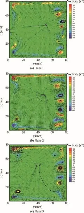
Fig.8 Variations of secondary flow along streamwise direction with Re=4750,Ro=0.25.

To explain all these phenomena mention above,an analysis method based on circulation was applied.By the way,the analysis below is based on some not-measured quantities,thus the explanation is essentially a speculation.Nevertheless,this analysis method provides a way to understand the physics nature behind the complex phenomena.The governing equation of circulation in the rotation coordinate is

Fig.9 Variations of secondary flow along streamwise direction with Re=4750,Ro=0.50.

Here,σ represents the relative density change and can be neglected in the present work.Moreover,the largest component of ▽2U is the x-component d2U/d y2.Thus,if δr was a vector in the cross-section plane,the viscous term can also be neglected.Consequently,Eq.(1)is reduced to

Eq.(2)means that the change of the circulation of a closed material line with time is the result of Coriolis force.

Based on Eq.(2),the reason why the disorderly arranged small vortices merge into orderly arranged large vortices is given as follow.The closed material lines which are also the paths of integral were chosen as shown in Fig.10,in which the ellipses represent the streamline of the vortex pair.In addition,there are two rectangular paths of integral.The hollow arrow one is related to the vortex with negative vorticity,and the solid arrow one is related to the vortex with positive vorticity.

At the edges of the rectangle parallel to the trailing side wall,the integral of Coriolis force is zero,because the Coriolis force is perpendicular to the trailing side wall.Meanwhile,at the edges of the rectangle perpendicular to the trailing side wall,the Coriolis force induced by the velocity of the primary flow will be different.That’s because on one hand,in the symmetrical line of the vortex pair,the vortex will push the low speed fluid near the trailing side away from the wall,thus reducing the velocity of the primary flow.On the other hand,at the other two edges parallel to the symmetrical line,the vortex will push the high-speed fluid at the edge of the boundary layer to the trailing side wall.As a result,the velocity of the primary flow will be enlarged.The averaged velocity in the symmetrical line is defined as Ulow,while the averaged velocity at the top edge and the bottom edge are defined as Uhigh.At this point,the hollow arrow integral can be expressed asand the solid arrow integral can be expressed as

for the vortex with negative vorticity.Integrating Eq.(3),there is

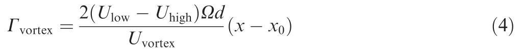
Here,Uvortexdenotes the averaged velocity of the primary flow in the region surrounded by the path of integral;Γvortexdenotes the circulation calculated along the path of integral that surrounds the vortex;x0denotes the x coordinate of the inlet.Similarly,there is

for the vortex with positive vorticity.

Fig.10 Path of integral for trailing side vortex pair.

According to Eqs.(4)and(5),it is not difficult to find that Γvortexdecreases with x for the vortex with negative vorticity and increases with x for the vortex with positive vorticity.Owing to the equality between the circulation and the area integral of the vorticity,it can be inferred that the absolute values of vorticity flux of both vortices increase with x.It is worth noting that the deduction above is based on the assumption that there is no vortex merging taking place.As the small vortices grow up along the streamwise direction and the width of the channel is limited,the merging of them is inevitable.

As for the reason of the differences between the high rotation number case and the low rotation number case,it will be discussed in the next section since it is related to rotation number.

4.4.Effects of rotation number

Fig.11 shows the variations of secondary flow fields with rotation number.The measurements were conducted at Plane 2 with Re=4750.The major effect of the rotation number on the secondary flow pattern is that,with the increase of rotation number,the merging of the trailing side roll-cells is evident.At the same time,the leading side vortices gradually become smaller and eventually disappear.The merging of the roll-cells near trailing side can also be explained by Eqs.(4)and(5).With the same streamwise position and Reynolds number,the absolute values of vorticity flux of the roll-cells near trailing side increase with rotation speed,namely the rotation number.For the same reason mentioned at the end of Section 4.3,the merging is inevitable.

As for the variations of the leading side vortices,the circulation analysis method was also adopted.

Fig.12 shows the integral path used in the analysis.The difference between the hollow arrow path and the solid arrow path is that top edge of the hollow arrow path is the top side wall,while that of the solid arrow path is the exterior edge of the Ekman layer.

The integral in Eq.(2)was first calculated along the hollow arrow,and the result is 2UcenterΩd,where Ucenterdenotes the averaged velocity of the primary flow in the symmetrical line.According to the derivation of Eqs.(3)and(4),there is

Here,Utophalfrepresents the averaged velocity for the top half of the channel.Γtophalfdenotes the circulation calculated along the hollow arrow of integral in Fig.12.Apparently,Γtophalfwill always be positive in the channel,and it increases with rotation number for the same position.

Then,the integral in Eq.(2)was calculated along the solid arrow,and there is

Here,Unon-Ekmandenotes the averaged velocity of the primary flow in the top half of the channel without the Ekman layer.UEkmandenotes the averaged velocity of the primary flow in the edge of the top side Ekman layer.Due to the Ekman pumping effect,UEkmanwill always be larger than Ucenter,thus Γnon-Ekmanwill always be negative in the channel,and decreases with rotation number for the same position.It can be inferred that the vorticity flux of the top side Ekman layer will always be positive and increases with rotation number,because it is equal to Γtophalf- Γnon-Ekman.However,this conclusion does not agree with the experimental results very well.This can be attributed to the bad particle image quality near the top side,which is induced by the laser light scattered by the top side wall.

Fig.11 Variations of secondary flow fields with rotation number.

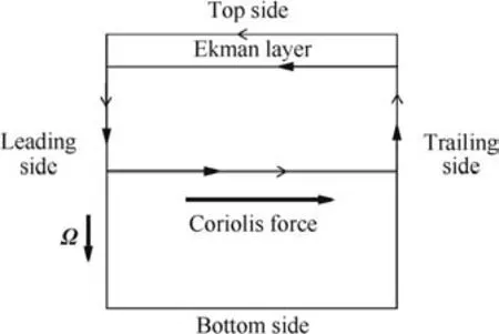
Fig.12 Integral path for upper part of channel.

Based on the above conclusions,the reason why the leading side vortices continuously diminish with rotation number is given here.Owing to the equality between the circulation and the area integral of the vorticity,the vorticity flux in the top half of the channel without the Ekman layer will always be negative in the channel,and it decreases with rotation number for the same position.When Re=4750 and Ro=0.25,as shown in Fig.11(a),there are exactly two trailing side vortex pairs in this region.The net vorticity flux of these two vortex pairs is close to zero because the positive vorticity flux may exactly cancel the negative vorticity flux out.As a result,the negative net vorticity flux of this region is provided by the vortex with negative vorticity near the leading side wall,since the associated vortex of it,which has positive vorticity,is almost in the Ekman layer.That means the vorticity flux of the associated vortex cannot be counted in.However,when Re=4750 and Ro=0.5,an important change takes place near the trailing side wall.There are only three,not four,vortex pairs near the trailing side for this case.The direct consequence of the change in the vortex pair number near the trailing side wall is that there is one more single vortex which has negative vorticity and is not cancelled out by the associated vortex in the region surrounded by the solid arrow of integral,as shown in Fig.11.According to Eq.(7),the net vorticity flux in the region surrounded by the solid arrow of integral for the case Ro=0.50 is twice as much as that for the case Ro=0.25.Therefore,if the absolute value of vorticity flux of the single trailing side vortex for the case Ro=0.50 was larger than that of the single leading side vortex for the case Ro=0.25,the absolute value of vorticity flux of the single leading side vortex for the case Ro=0.50 will be less than that for the case Ro=0.25.This means the merging of the trailing side vortices can induce the diminishing of the leading side vortices.Thus,it can be concluded that the secondary flow filed has to be treated as a whole.

This can also be used to explain the differences between the development of the leading side vortices for the high rotation number case and that for the low rotation number case.Apparently,there are four trailing side vortex pairs for the low rotation number case,as shown in Fig.11(a).However,this number changes to three for the high rotation number case,as shown in Fig.11(b).According to Eq.(7),Γnon-Ekman,namely the vorticity flux in the region surrounded by the solid arrow of integral shown in Fig.12 will always be negative in the channel,and it decreases with x for the same rotation number.On one hand,when Ro=0.25,namely there are four trailing side vortex pairs,the decrease of Γnon-Ekmanis mainly realized by the strengthening of the leading side vortices,especially the vortex with negative vorticity.On the other hand,when Ro=0.50,namely there are only three vortex pairs near the trailing side,the decrease of Γnon-Ekmanis mainly realized by the strengthening of the trailing side vortex which is not cancelled out.Thus,the leading side vortex with negative vorticity weakens along the streamwise direction.

4.5.Effects of Reynolds number

Fig.13 shows the development of secondary flow fields along the streamwise direction with the same rotation number(Ro=0.25)and different Reynolds number(Re=4750,9500).

Obviously,the trailing side vortices for the higher Reynolds number case are stronger than those for the lower Reynolds number case.The reason is discussed from the perspective of Coriolis instability,since the trailing side vortices are induced by the Coriolis instability.

Bradshaw30proposed to use Richardson number to depict the strength of Coriolis instability.The definition of Richardson number is

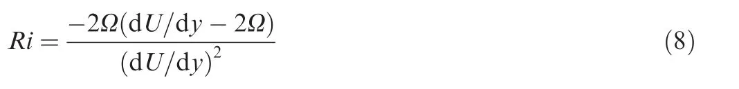
Fig.13 Secondary flow fields with different Reynolds number.

When Ri＜0,the Coriolis force makes the boundary layer unstable.And,smaller Richardson number means stronger Coriolis instability.It is worth mentioning that Richardson number is a normalized parameter to characterize the strength of Coriolis instability,whereas the corresponding primitive parameter should be-2Ω（d U/d y-2Ω）.Since the strength of the trailing side vortices are described by vorticity,which is a primitive parameter,thus-2Ω（d U/d y-2Ω）is used as a measure of the Coriolis instability.

For the higher Reynolds number case(Re=9500),it can be inferred that d U/d y and Ω are roughly twice as much as those of the lower Reynolds number case.Moreover,in the boundary layer near trailing side,d U/d y-2Ω＞0.So,d U/d y-2Ω for the higher Reynolds number case is larger than that for the lower Reynolds number case.Meanwhile,-2Ω（d U/d y-2Ω）for the higher Reynolds number case is less than that for the lower Reynolds number case.That’s to say,the higher Reynolds number case has stronger primitive Coriolis instability,thus has stronger trailing side vortices.

As for the leading side vortices,the higher Reynolds number case has larger vorticity in Plane 1 and Plane 2.However,the opposite situation takes place in Plane 3.

Similarly,the circulation analysis method can be used to explain the results measured in Plane 1 and Plane 2.According to Eq.(7),the strength of the leading side vortices is proportional to the product ofand Ω when the number of trailing side vortex pairs is even.Although it is difficult to estimate in which caseis larger,the rotation speed for the higher Reynolds number case is double of the lower one.In general,the product ofand Ω is larger for the higher Reynolds number case.

In addition,the reason for the reversal is that the merging of the trailing side vortices happened between Plane 2 and Plane 3 for the case Re=9500,and the number of the vortex pairs near trailing side changes from four to three.This explanation indicates that the increase of Reynolds number makes the merging of the trailing side vortices occur upstream,and the underlying cause is the increase of the primitive Coriolis instability with Reynolds number.

5.Conclusions

The development of the secondary flow field in a rotating square cross-section straight channel was experimentally measured by PIV.The inlet mean velocity of the channel was approximately irrotational,and the turbulence intensity was about 1%.Thus,in the stationary cases,the boundary layer flow was still laminar.The experiments were conducted with different streamwise positions,rotation numbers and Reynolds numbers to find the effects of these parameters on the development of the secondary flow field.To minimize the measurement error due to the relative movement between the rotating channel and the stationary PIV system,an FPGA based trigger signal generator was developed.Due to intrinsic limit of the measurement method,the accuracy of the velocity was very low in the core region,so the discussion is limited at the locations where the relative error is acceptable.And the following conclusions are given:

First,the absolute values of vorticity flux of the roll cells near the trailing side increases with increasing radius of the measured plane and rotation number.When the absolute value of vorticity flux exceeds a critical value,the merging of the trailing side roll cells appears.

Moreover,when the number of the trailing side vortex pairs is even,the absolute value of vorticity flux of the vortices in the leading side corner region increases along streamwise direction.Otherwise,the absolute value of vorticity flux decreases along the streamwise direction.By the circulation analysis,the authors found that this phenomenon has relationship with the merging of the trailing side roll cells,and further concluded that the secondary flow field in a rotating channel has to be treated as a whole.

At last,the increase of the Reynolds number was found to be able to induce the merging position moves upstream.

Acknowledgements

The present work is financially supported by the Academic Excellence Foundation of BUAA for Ph.D.students,and the National Natural Science Foundation of China (No.51506002).