DYNAMICAL ANALYSIS OF A SINGLE-SPECIES POPULATION MODEL WITH MIGRATIONS AND HARVEST BETWEEN PATCHES∗†
2018-07-06ChenjiaWangFengyingWei
Chenjia Wang,Fengying Wei,2‡
(1.College of Math.and Computer Science,Fuzhou University,Fuzhou 350116,Fujian,PR China;
2.Key Laboratory of Operations Research and Control of Universities in Fujian,Fuzhou University,Fuzhou 350116,Fujian,PR China)
1 Introduction
The environmental pollution and the unregulated harvesting/hunting threaten the life of wild animals and the biological diversity.In order to prevent the biological resources from destruction and to protect the ecological environment,the human beings therefore have taken various measures to deal with these situations.The most and popular measure is to establish the protection zone to the endangered species in the recent decades.
The species with the unregulated harvest from human beings have been paid more attention by the researchers,and the related improvements have been derived by various techniques.Within recent two decades,the models with protection zones have been investigated by the researchers and scholars around the world,where the single-species population models were focused on in[1-5],the predator-prey models were studied in[6-9]and the competitive model was considered in[10].Among these results,the stability and optimal harvest of the corresponding models were presented in[1-3],and the diffusion or migration-dependent models were extensively discussed in[1-10].We would like to mention the work by Fan and Wang[1],in which they considered a model on harvested population with diffusion migration:

where x(t)is the density of the species in the natural environment and y(t)is the density of the same species in the natural reserve at time t,respectively;r is the intrinsic growth rate;K is the carry capacity of the environment.The item d(x(t)−y(t))represents the diffusion capacity that is the total biomass caused by the diffusion effect,where d is the proportional coefficient and is assumed to be proportional to the difference of the densities.
According to the reports from the statisticians and the official investigations by the forestry of China,for the endangered species,the density of most species in the natural environment(also called the unprotected patch,non-protection zone)is less than the density in the natural reserve(also called the protected patch,protection zone),such as the Tibetan antelopes,the Asian elephants and other rare species.However,food-dependent and/or temperature-dependent distributions of the species,the plenty of food source and health care are the main factors for the species to migrate from one patch to another.That is,the diffusion of the species is actually a double-direction process between two patches.We denote the immigration rate from the unprotected to protected patch by m1,and the emigration rate from the protected to unprotected by m2,instead of one-direction diffusion process of model(1).And we also assume that m1≥m2throughout this paper.
When it comes to the financial benefit of the species,the hunters generally take high risk to harvest the individuals in the unprotected patch.Throughout this paper,we always assume that E1and E2are the hunting rates in the unprotected area and protected patch,respectively.Besides,we also assume that the hunting rate in the protective patch is much lower than that in the unprotected area,that is,E2≪E1.The previous model(1)could be improved as

which turns to model(1)when m1=m2=d and E2=0 in model(2).
In the next section,we will discuss the local and global stability of the equilibria by means of Jacobian matrix and phase plane analysis.And in Section 3,we will investigate the practical effects of the protection zone and harvest regarding the conservation of population resources,and several controllable and efficient strategies are proposed to the local management centers.A numerical simulation is given in Section 4.We end this paper with a conclusion.
2 Global Analysis of the Equilibria and Their Stability
In this section,we will study the dynamical behaviors of model(2)and analyze the existence and stability of the equilibria.Let

Now,substituting(3)into(2),removing the primes,still and using the symbols proposed in model(2),we rewrite model(2)as

whereα=≥1,x(t)and y(t)denote the densities of the species in the unprotected and protected patches at time t,respectively.Therefore,we only need to study model(4)in the region

The equilibria of model(4)are the solutions of the following equations

We attempt to investigate the stability of the origin of model(4)by means of Jacobian matrix,and the existence and stability of the positive equilibria of model(4)in the phase plane as well.It is obvious that O(0,0)is an equilibrium of model(4).Next we will analyze the stability of O(0,0)in Theorem 2.1.
The Jacobian matrix of the linearized model of(4)at O(0,0)is given by

Eigenvalues of J(0,0)satisfy

that is,

where

Solving(8)produces

which also implies

The solution ofλ+λ−=0 is given by

From λ++λ−=0,we obtain that

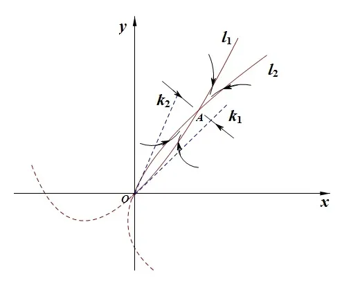
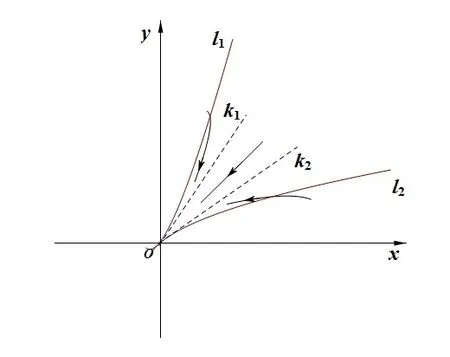
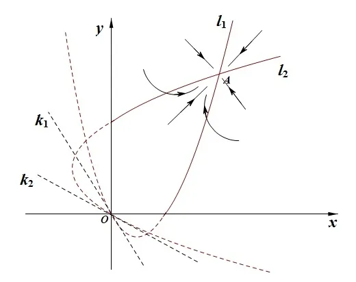
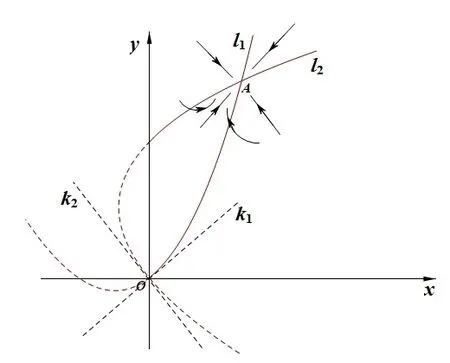
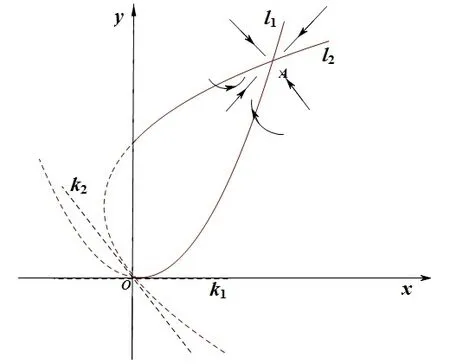
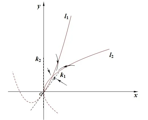
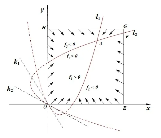
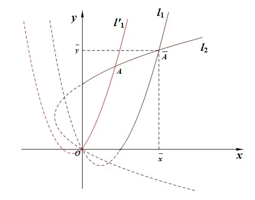
It is easy to check that 0 Theorem 2.1Ifr1 ProofIf r1 which implies that Therefore,O(0,0)is a saddle point. If 0 and which leads toλ±<0.We can conclude that O(0,0)is a stable node. If r>r2,then and which meansλ±>0.Hence O(0,0)is an unstable node.The proof is complete. The positive solution of(6)is a positive equilibrium of model(4),which is also the intersection in the positive quadrant of the following two isoclines: We denote the upward parabola by l1with its symmetric line x=and the right parabola by l2with its symmetric line y=Also denote the positive equilibrium of system(4)by A(x∗,y∗).And,the positive equilibrium A(x∗,y∗)is the only intersection of the graphs y=g1(x)and x=g2(y)in the region D. Definition 2.1[1]The left-component(or the right-component)of l1is defined as the set composed of points lying in Definition 2.2[1]The upper-component(or the lower-component)of l2is defined as the set composed of points lying above(or under)the line Obviously,the tangent pointis on the right-component of l1(the upper-component of l2)if and only if the slope of the tangent line of y=g1(x)(x=g2(y))is positive.And,the tangent point is on the left-component of l1(the lower-component of l2)if and only if the slope of the tangent line of y=g1(x)(x=g2(y))is negative. Theorem 2.2If the following conditions holds,then model(4)admits a unique positive equilibriumA(x∗,y∗)with0 hold,then model(4)has no positive equilibrium;in this case,A(x∗,y∗)degenerates to the unique equilibriumO(0,0)in the regionD. ProofLet ki(i=1,2)denote the slopes of the tangent lines of li(i=1,2)at O(0,0),we then easily get that We set then x∗satisfies the equation F(x)=0,and The right-component of l1and the upper-component of l2intersect at O(0,0)and the positive equilibrium A(x∗,y∗)of model(4)if the two slopes satisfy the condition 0 Figure 1:0 The expression(26)demonstrates that the slopes k1and k2of the tangent lines of l1and l2at O(0,0)respectively depending on E1and E2.According to the general assumption E1≫E2of this paper,k1increases if E1increases linearly and continuously with respect to E1,while k2decreases slightly with small increment of E2with the fixed constantsαand r,that is,k2can be regarded as an invariant constant when the increment of E2is very small. If then the slopes of two curves satisfy k1>k2>0,which implies that the right component of l1lies above the upper-component of l2.We can check that if condition(31)is satisfied,then positive equilibrium A(x∗,y∗)gradually vanishes and finally degenerates to the origin O(0,0). If is valid,then the positive equilibrium A(x∗,y∗)coincides with O(0,0),also l1and l2are respectively tangent at O(0,0).The positive equilibrium A(x∗,y∗)approaches O(0,0)continuously along the upper-component of parabola l2lying in the first quadrant as shown in Figure 2. Figure 2:0 Case 3r>α+E1. The left-component of l1and the lower-component of l2intersect at O(0,0),and the positive equilibrium A(x∗,y∗)of model(4)exists if the two slopes satisfy the conditions ki<0(i=1,2).By the similar discussion,we can easily reach the conclusion that A(x∗,y∗)is a unique positive equilibrium of model(4)with 0 Figure 3:r>α+E1 Case 41+E2≤r≤α+E1. Obviously,the slopes of two curves satisfy k1>0 and k2<0 if 1+E2 Figure 4:1+E2 The special case is k1=0 and k2<0 if r=α+E1,which is presented in Figure 5.Similarly,the slopes satisfy k1>0 and k2=∞if r=1+E2.In this subcase,the curve l2is tangent to the y-axis at O(0,0)and is symmetric to the x-axis.By the same argument,there exists a unique positive equilibrium as demonstrated in Figure 6. Figure 5:r=α+E1 with k1=0 Figure 6:r=1+E2 with k2=∞ Through the discussions from Case 1 to Case 4,we could present the existence and uniqueness of the positive equilibrium A(x∗,y∗)under some sufficient conditions.Next,we will aim at the stability of the positive equilibrium A(x∗,y∗). The Jacobian matrix of the linearized system of(4)around A(x∗,y∗),together with equalities(6),can be written as then the eigenvalues λi(i=1,2)of J(x∗,y∗)satisfy where the product and sum of these two eigenvalues are respectively Hence,λ1<0,λ2<0,which implies that A(x∗,y∗)is a stable node.The proof of Theorem 2.2 is complete. Remark 2.1Figure 1 and Figures 3-6 demonstrate the positions of the positive equilibrium A(x∗,y∗)to model(4).And,the isoclines and involved trajectories close to A(x∗,y∗)explain how the dynamical behaviors undertake within the first quadrant,where A(x∗,y∗)is stable and attracts all trajectories of model(4),and O(0,0)is unstable.While Figure 2 shows that model(4)does not admit any positive equilibrium except for O(0,0),which is the unique stable equilibrium within the first quadrant.For each species in both patches,the density is always expected to be extinct. Theorem 2.3Each trajectory of model(4)issuing fromDis always positive and bounded. ProofTo end this,we denoteby the outward normal of the closed boundary,and(˙x,˙y)by the vector pointing inwards for all points on the boundary.Now,we must find a simple closed boundary curve in D such that the phase trajectories starting from the boundary always point inwards.According to the signs of f1(x,y)and f2(x,y),the angle between the vectorand outward normalis an obtuse angle as demonstrated in Figure 7.If the trajectory issues from the boundary,then it will run inwards along the vector.And if it does reach the boundary,the vectordoes not allow the trajectory to move outwards.We could claim that no trajectory can leave the domain D if it is once inside. Let us,for example,only aim at the case(24).Other cases can be proved by the similar arguments.It is not difficult to see that,under condition(24),the direction of the vectorand the direction of the(x,y)trajectory is governed by the signs of vector components(f1(x,y)and f2(x,y))as shown in Figure 7. Figure 7:Nulllines f1(x,y)=0,f2(x,y)=0 for system(4)under condition(24). We assume that(x(t,x0),y(t,y0))is the trajectory of system(4)starting from(x0,y0)for any fixed(x0,y0)∈D.We can draw a straight line parallel to the y-axis from point E(x0+1,0),which intersects the parabola l2at F(x0+1,y1),where Again,we draw a straight line parallel to the x-axis from point G(x0+1,y2),and denote the intersection of the straight line and y-axis as H(0,y2),where y2=max{y1,y0+1}.Therefore,we construct a bounded closed set O E F GH O.The trajectory(x(t,x0),y(t,y0))can not leave the region O E F GH O because the direction of the vectorpoint inwards on the boundary.That is,the trajectory(x(t,x0),y(t,y0))is positive and bounded.The proof is complete. Remark 2.2The region O E F GH O is a bounded closed set on which the trajectories all point inwards due to the fact<0,whereis the unit outward normalon the boundaries.The direction of the vectoris determined by the signs of f1and f2,which could be found on either side of the nulllines. We then derive two main theorems without proof. Theorem 2.4Ifthen the unique positive equilibriumA(x∗,y∗)of model(4)is globally asymptotically stable. Theorem 2.5If then the unique equilibriumO(0,0)of model(4)is globally asymptotically stable. We attempt to investigate the practical effects with respect to the protected patch and harvesting,and the discussion will be separated into two cases. Case 1r≥1+E2,that is,r≥m2+E2in model(2). If E1=0,E2=0,then the positive equilibrium A(x∗,y∗)turns to the point A¯(x¯,y¯),which is the intersection of l1and l2in the positive quadrant,whereA¯(x¯,y¯)satisfies the equalities We increase the harvesting rates E1and E2simultaneously from 0.Together with the assumption E2≪E1,the increment of E2is always regarded as a tiny variation compared with the increment of E1within the same time scale,which is demonstrated in Figure 8.The curve l2can be regarded as a sort of fixed curve due to its tiny change,while the curve l1gradually moves to a new curve. Figure 8:Nulllines f1(x,y)=0,f2(x,y)=0 for system(4)when r>1+E2 and E1 increases. The x-coordinate of the intersection of the curveand the straight line y=is expressed by which decreases as E1increases.We observe from Figure 8 that,the x-coordinate of the intersection ofand l2decreases gradually.We consequently find that which means that the density of the species in the unprotected patch declines to a very low level when the harvesting effort is large enough.Together with the expression(41),one easily derives that which represents that the density of the species in the protected patch approaches a fixed constant 1−under a long time running. When we take a fixed harvesting level,Theorem 2.4 indicates that all trajectories of model(4)definitely tend to the equilibrium A(x∗,y∗),which means that the protected patch can efficiently eliminate the extinction of the species when over harvesting takes place. If there is no protection zones for the species,that is,the migration rates m1and m2are removed from the original model(2),then the species might be easily extinct under a catastrophes harvesting E1≥r.On the contrary,if there exist protection zones,by expression(44),1−is equivalent to 1−of the originalmodel(2).For the species in the protected patch,the smaller the emigration rate m2is,the higher density of the species has.In order words,the protection zones indeed eliminate the extinction of the species. Case 20 If 0 holds,the positive equilibrium A(x∗,y∗)vanishes and degenerates to a unique globally asymptotically stable equilibrium O(0,0).In this case,all trajectories tend to O(0,0)as time t approaches infinity.Clearly,the harvesting really leads to the extinction of the species within two patches. Theorem 2.4 shows that alltrajectories of model(4)issuing from D tend to the unique positive equilibrium A(x∗,y∗)as time goes to infinity,and the species will never be extinct in this case under condition When we increase E1to the right boundary from the left then x∗and y∗decrease monotonically,and one gets that The above discussions indicate that the threshold of the extinction to the species exists.When E1exceeds the threshold,the species within two patches are definitely extinct,otherwise the densities of the species are kept as constant levels x∗and y∗respectively,which means the protected patches really improve the persistence of the biological resources. Combing Case 1 with Case 2,we point out that the extinction of the species is unavoidable under some extreme conditions(40).Meanwhile,the establishment of the protection zones does prevent the species from dying out or does slow down the extinction under condition(38)or(39).That is,the protection zones are beneficial to the enhancement of the density to the endangered species,and also good for the diversity of the species.For the practical managements,the improvement of the punishment strength is necessary in order to restrict the harvesting,and setting simple obstacles on the boundaries of the protection zones is effective in order to eliminate the migrations. We set the parameters of model(4)as follows: and the initial value is(x0,y0)=(2,3).We can easily verify thatα=>1,0 Figure 9:0 Figure 10:r≥ 1+E2 In this paper,we present a model of single-species population with migrations and harvest between the protected patch and the unprotected patch.Then,we investigate the dynamical behavior of the population and analyze the existence and stability of the equilibria.Our research points out,model(2)admits a unique positive equilibrium,which is globally asymptotically stable under condition(38)or(39).Further,if condition(40)is satisfied,the unique positive equilibrium of model(2)degenerates to O(0,0),which is globally asymptotically stable.We also discuss the practical effects of the protection zones and draw the conclusions regarding model(2)that:When r≥m2+E2,the protection zone can effectively eliminate the extinction of the population;if E1→∞,the population level within the unprotected zone tends to zero,and the population level within the protected zone tends to 1−;when 0 the population within two patches becomes extinct. In the practical management of the protection zones,an effective method for eliminating the possibility of extinction is to set simple obstacles on the boundaries aiming at reduction of migration rates,and to enhance the supervision of human being aiming at reduction of hunting rate.Our practical strategies might apply to the species including Tibetan antelope and Asian elephants to avoid the extinction of the population within protected zones.And,we will organize another research paper to investigate the dynamical properties of single-species population with random perturbations in the future. [1]M.Fan,K.Wang,Study on harvested population with diffusional migration,Journal of Systems Scicence and Complexity,14:2(2001),139-148. [2]T.K.Kar,H.Matsuda,A bioeconomic model of a single-species fishery with a marine reserve,Journal of Environmental Management,86(2008),171-180. [3]Eduardo Gomzález-Olivares,Jiame Huincahue-Arcos,A two-patch model for the optimal management of a fishing resource considering a marine protected area,Nonlinear Analysis:Real World Applications,12(2011),2489-2499. [4]X.Zou,K.Wang,The protection zone of biological population,Nonlinear Analysis:Real World Applications,12(2011),956-964. [5]X.Zou,K.Wang,M.Liu,Can protection zone potentially strengthen protective effects in random environments?Applied Mathematics and Computation,231(2014),26-38. [6]Y.Du,J.Shi,A diffusive predator-prey model with a protection zone,Journal of Differential Equations,229(2006),63-91. [7]Y.Lv,R.Yuan,Y.Pei,A predator-prey model with harvesting for resource with reserve area,Applied Mathematical Modelling,37(2013),3048-3062. [8]H.Yang,J.Jia,Harvesting of a predator-prey model with reserve area for prey and in the presence of toxicity,Journal of Applied Mathematics and Computing,53(2017),693-708. [9]X.He,S.Zheng,Protection zone in a diffusive predator-prey model with Beddington-DeAngelis functional response,Journal of Mathematical Biology,75(2017),239-257. [10]Y.Du,X.Liang,A diffusive competition model with a protection zone,Journal of Differential Equations,244(2008),61-86.








3 Practical Effects of the Protected Patch and Harvest



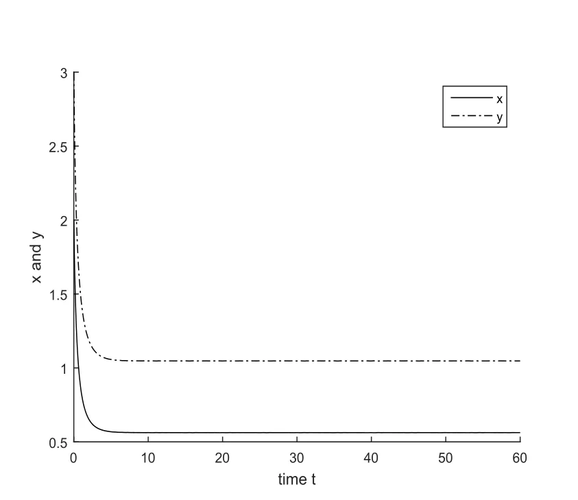
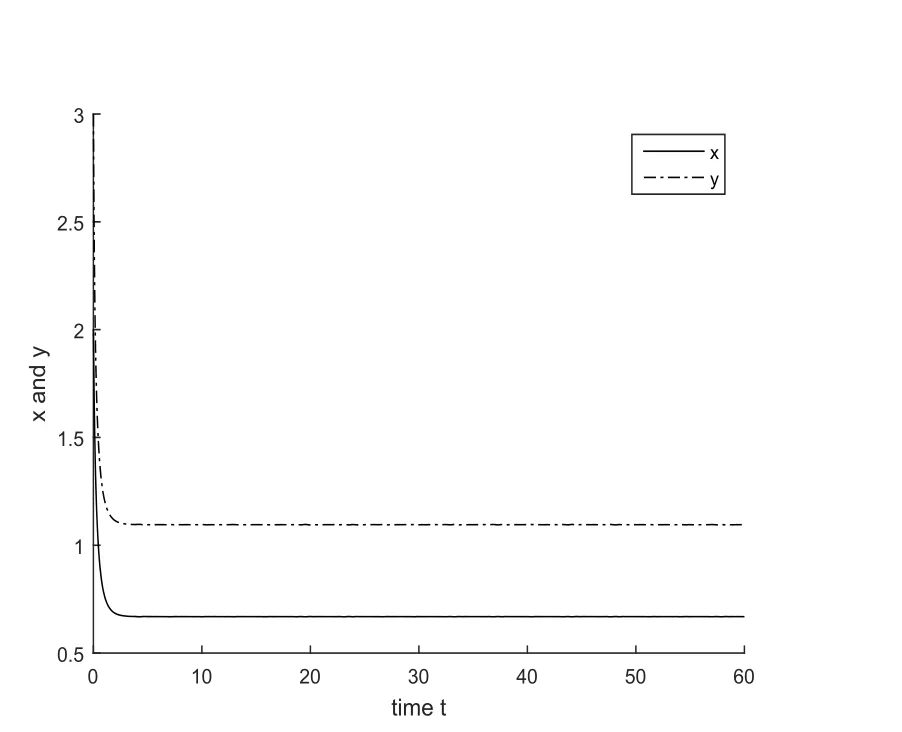
4 Numerical Simulation

5 Conclusion and Discussion

杂志排行
Annals of Applied Mathematics的其它文章
- DYNAMICS OF A PREDATOR-PREY REACTION-DIFFUSION SYSTEM WITH NON-MONOTONIC FUNCTIONAL RESPONSE FUNCTION∗†
- THE BOUNDS ABOUT THE WHEEL-WHEEL RAMSEY NUMBERS∗
- NEWDYNAMICINEQUALITIES FORDECREASING FUNCTIONS AND THEOREMS OF HIGHER INTEGRABILITY∗
- A COMMENSAL SYMBIOSIS MODEL WITH HOLLING TYPE FUNCTIONAL RESPONSE AND NON-SELECTIVE HARVESTING IN A PARTIAL CLOSURE∗†
- A BLOCK-COORDINATE DESCENT METHOD FOR LINEARLY CONSTRAINED MINIMIZATION PROBLEM∗†
- ESTIMATION OF PARAMETERS IN A CLOSED PYGMY POPULATION IN CAMEROON∗†
