New Double-Periodic Soliton Solutions for the(2+1)-Dimensional Breaking Soliton Equation∗

2018-06-11JianGuoLiu刘建国andYuTian田玉

Communications in Theoretical Physics 2018年5期

关键词：刘建国

Jian-Guo Liu(刘建国) and Yu Tian(田玉)

1School of Science,Beijing University of Posts and Telecommunications,Beijing 100876,China

2School of automation,Beijing University of Posts and Telecommunications,Beijing 100876,China

3College of Computer,Jiangxi University of Traditional Chinese Medicine,Nanchang 330004,China

1 Introduction

Nonlinear evolution equations(NLEEs)are frequently used to model a wide variety of nonlinear scientific phenomena,such as marine engineering, fluid dynamics,plasma physics,chemistry,physics and so on.Direct seeking for exact solutions to NLEEs has become one of the most exciting and extremely active areas in mathematical physics.[1−23]In the past few decades,with the development of symbolic computation,many powerful and systematic methods have been proposed,such as Hirota direct method,[24]F-expansion method,[25]exp function method,[26−28]the auxiliary equation method,[29]three wave approach[30−36]and etc.

The breaking soliton equations can be applied to describe the(2+1)-dimensional interaction of a Riemann wave propagating along the y-axis with a long wave propagating along the x-axis.[37]In this paper,we will discuss the following(2+1)-dimensional breaking soliton equation:[37−41]

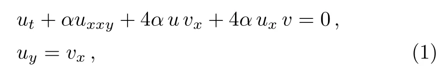
where α is an arbitrary constant. Radaha and Lakshmanan have proved that Eq.(1)has the Painlev´e property and dromion-like structures.[38]The folded solitary waves and other coherent soliton structures are discussed.[39−40]By introducing Jacobi elliptic functions in the seed solution,two families of doubly periodic propagating wave patterns are obtained.[37]Exact breathertype and periodic-type soliton solutions for the(2+1)-dimensional breaking soliton equation are derived via the extended three-wave method.[41]

However,to our knowledge,double-periodic soliton solutions for Eq.(1)have not been discussed,which turn out to be the main goal of the present work.In Sec.2,new double-periodic soliton solutions for Eq.(1)are researched by virtue of the symbolic computation,bilinear form and the special ans¨atz functions.Finally,Sec.3 will be the conclusions.

2 New Double-Periodic Soliton Solutions and Bilinear Form

Using the following dependent variable transformation

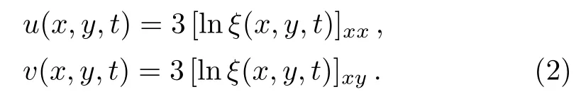
Substituting Eq.(2)into Eq.(1),the(2+1)-dimensional breaking soliton equation can be written in the following bilinear form

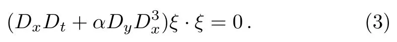
Equation(3)is equivalent to the following equation

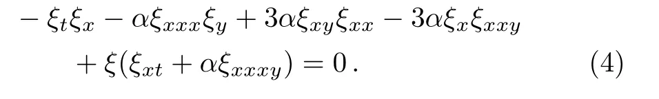
Supposing the solution of Eq.(4)be expressed in the form

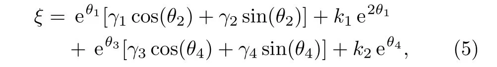
where θi= αix+ βiy+ δit,i=1,2,3,4 and αi,βi,and δiare constants to be determined later.Solution(5)is if rst proposed in the literature[36]for the purpose of solving the multi periodic soliton solutions of the Kadomtsev-Petviashvili equation.This method is simple and direct,and can obtain a large number of periodic solutions of the high dimensional nonlinear equations.But the amount of computation is large and the help of symbolic computing software Mathematica is needed.Substituting Eq.(5)into Eq.(4)and equating corresponding coefficients of eθ1,eθ3,eθ4,cosθ2,sinθ2,cosθ4,and sinθ4to zero,a set of algebraic equations for αi,βi,δican be derived as follows

Solving the system with the aid of symbolic computation software Mathematica,we have

Case 1

where α,α1,β1,β2,β3,β4,k2,γ1,γ2,γ3,and γ4are free real constants.Substituting these results into Eq.(5),we obtain

Therefore we obtain the fi rst new double-periodic soliton solutions for Eq.(1)as follows:

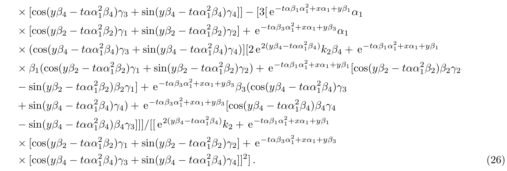
The evolution and mechanical feature of solutions(25)–(26)are shown in Figs.1–2.

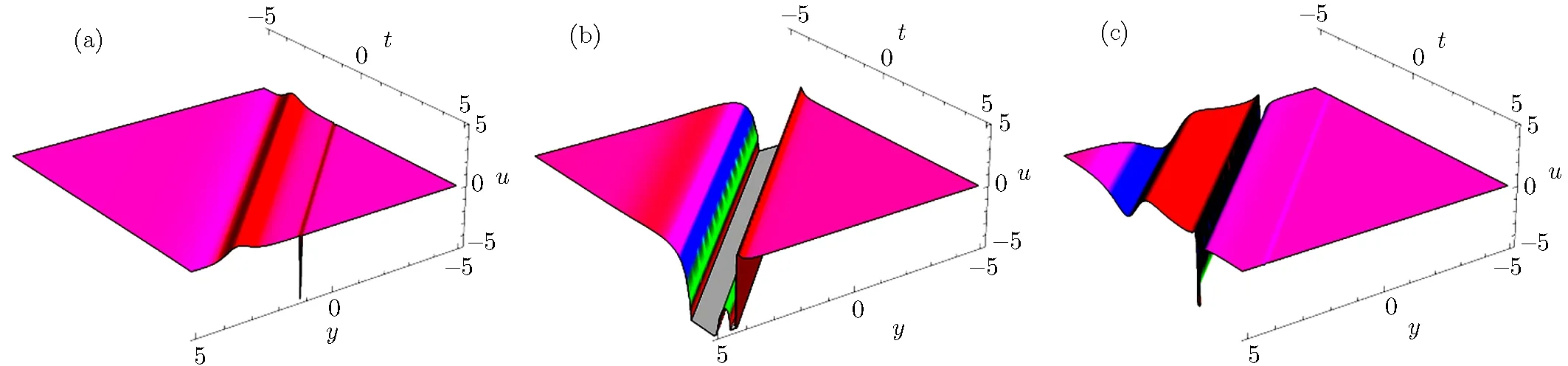
Fig.1 The physical structure of solution(25),at k2= β3= −1,α1= γ1=1,γ2= γ3= γ4= β1= β2= β4= α =1,(a)x=−5,(b)x=0 and(c)x=5.

Fig.2 The physical structure of solution(26),at k2= β3= −1,α1= γ1=1,γ2= γ3= γ4= β1= β2= β4= α =1,(a)x=−5,(b)x=0 and(c)x=5.

Case 2

where α,α1,β1,β2,β3,β4,k1,γ1,γ2,γ3,and γ4are free real constants.Substituting these results into Eq.(5),we obtain

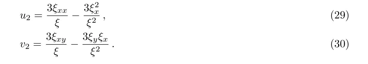
Therefore we obtain the second new double-periodic soliton solutions for Eq.(1)as follows:ξ has been explained in Eq.(28).The evolution and mechanical feature of solutions(29)–(30)are shown in Figs.3–4.

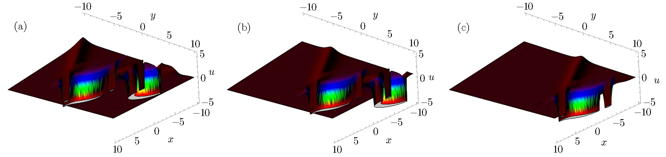
Fig.3 The physical structure of solution(29),at k1= β3= −1,α1= γ1=1,γ2= γ3= γ4= β1= β2= β4= α =1,(a)t=−5,(b)t=0 and(c)t=5.

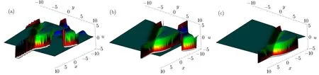
Fig.4 The physical structure of solution(30),at k2= β3= −1,α1= γ1=1,γ2= γ3= γ4= β1= β2= β4= α =1,(a)t=−5,(b)t=0 and(c)t=5.

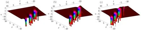
Fig.5 The physical structure of solution(33),at k1= β1= β3= −1,α1=1,γ1= γ2= γ3= γ4= β2= β4= α =1,(a)y=−5,(b)y=0 and(c)y=5.

Case 3

where α,α1,β1,β2,β3,β4,k1,γ1,γ2,γ3,and γ4are free real constants.Substituting these results into Eq.(5),we obtain

Therefore we obtain the third new double-periodic soliton solutions for Eq.(1)as follows:ξ has been explained in Eq.(32).The evolution and mechanical feature of solutions(33)–(34)are shown in Figs.5–6.

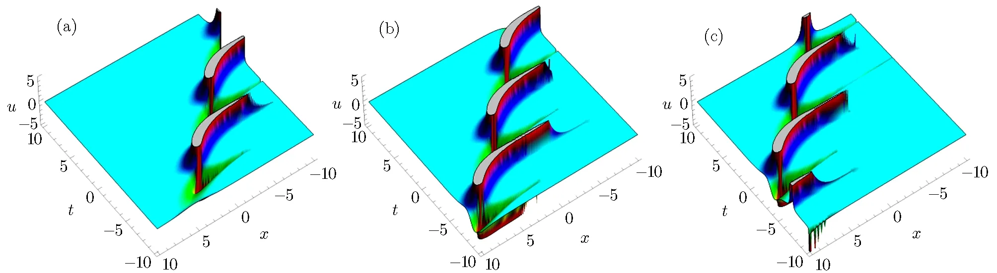
Fig.6 The physical structure of solution(34),at k1= β1= β3= −1,α1=1,γ1= γ2= γ3= γ4= β2= β4= α =1,(a)y=−5,(b)y=0 and(c)y=5.

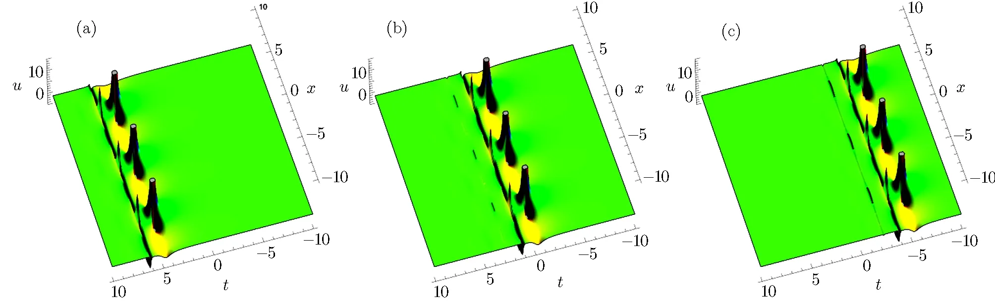
Fig.7 The physical structure of solution(37),at α2= γ1= β1= γ4= −1,β4= −2,k1= γ2= γ3= β3= α =1,(a)y=−5,(b)y=0 and(c)y=5.

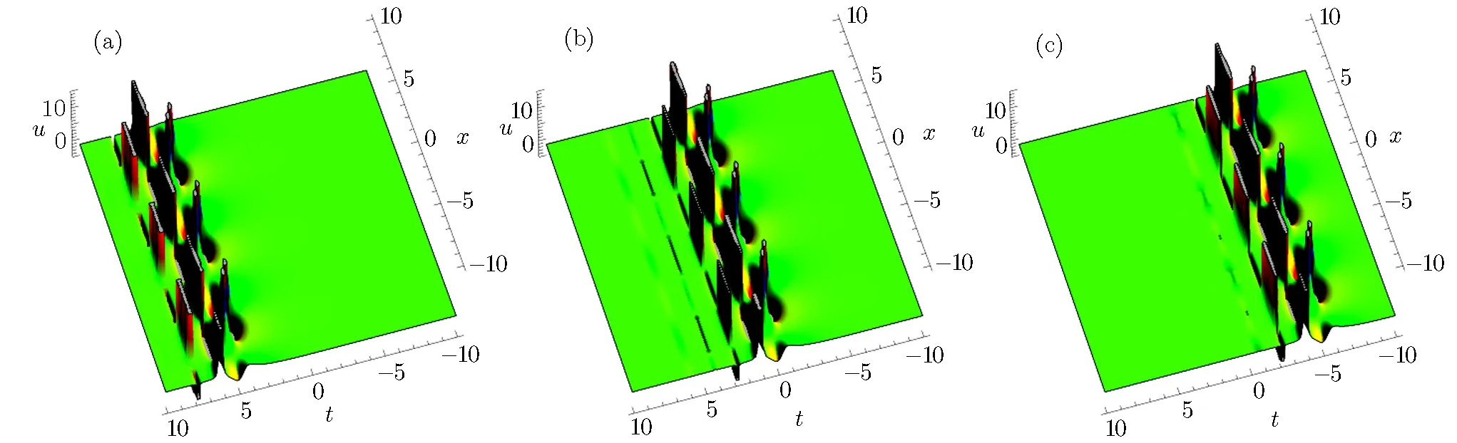
Fig.8 The physical structure of solution(38),at α2= γ1= β1= γ4= −1,β4= −2,k1= γ2= γ3= β3= α =1,(a)y=−5,(b)y=0 and(c)y=5.

Case 4

where α,α2,β1,β3,β4,k1,γ1,γ2,γ3,and γ4are free real constants.Substituting these results into Eq.(5),we obtain

Therefore we obtain the fourth new double-periodic soliton solutions for Eq.(1)as follows:

ξ has been explained in Eq.(36).The evolution and mechanical feature of solutions(37)–(38)are shown in Figs.7–8.

Case 5

where α,α1,α2,α3,β1,k2,γ2,and γ4are free real constants,ϵ1= ±1.Substituting these results into Eq.(5),we obtain

Therefore we obtain the fi fth new double-periodic soliton solutions for Eq.(1)as follows:

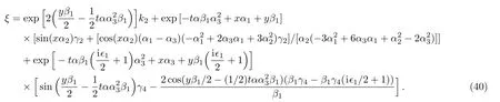
ξ has been explained in Eq.(40).

Case 6

where α,α1,α2,β1,β4,k2,γ2,and γ4are free real constants,ϵ2= ±1.Substituting these results into Eq.(5),we obtain

Therefore we obtain the sixth new double-periodic soliton solutions for Eq.(1)as follows:

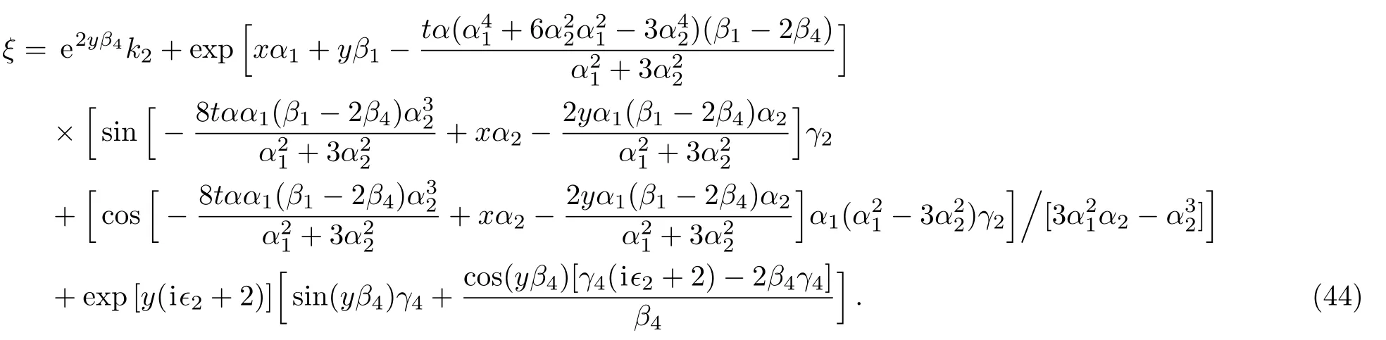
ξ has been explained in Eq.(44).

Case 7

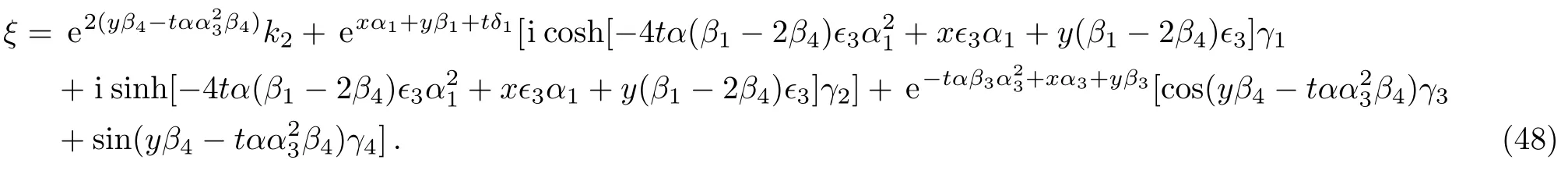
where α,α1,α3,β1,β3,β4,k2,γ2,γ3,and γ4are free real constants,ϵ3= ±1.Substituting these results into Eq.(5),we obtain

Therefore we obtain the seventh new double-periodic soliton solutions for Eq.(1)as follows:

ξ has been explained in Eq.(48).The evolution and mechanical feature of solutions(49)–(50)are shown in Figs.9–10.

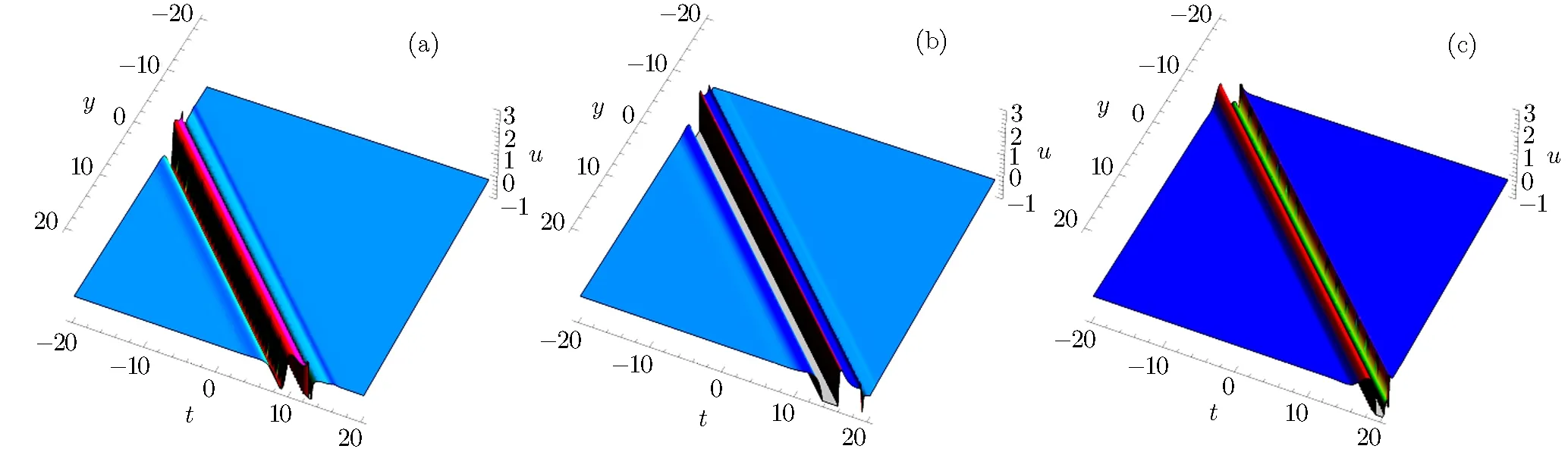
Fig.9 The physical structure of solution(49),at α3= γ2= β1= γ4= −1,k2= −2,γ3=2,α1= β3= β4= α = ϵ3=1,γ2=0(a)x=−10,(b)x= −5 and(c)x=−1.

Fig.1 0 The physical structure of solution(50),at α3= γ2= β1= γ4= −1,k2= −2,γ3=2,α1= β3= β4= α =ϵ3=1,γ2=0(a)x= −10,(b)x= −5 and(c)x= −1.

Case 8

where α,α1,α2,β1,β2,β3,β4,k2,δ2,γ1,γ3,and γ4are free real constants,ϵ4= ±1.Substituting these results into Eq.(5),we obtain

Therefore we obtain the eighth new double-periodic soliton solutions for Eq.(1)as follows:

ξ has been explained in Eq.(52).

Case 9

where α,α3,α4,β1,β2,β4,k2,δ2,γ2,and γ3are free real constants,ϵ5= ±1.Substituting these results into Eq.(5),we obtain

Therefore we obtain the ninth new double-periodic soliton solutions for Eq.(1)as follows:

ξ has been explained in Eq.(56).

Case 10

where α,α4,β1,β2,β3,β4,k1,k2,γ1,γ2,γ3,and γ4are free real constants.Substituting these results into Eq.(5),we obtain

Therefore we obtain the tenth new double-periodic soliton solutions for Eq.(1)as follows:

ξ has been explained in Eq.(60).The evolution and mechanical feature of solutions(61)–(62)are shown in Figs.11–12.

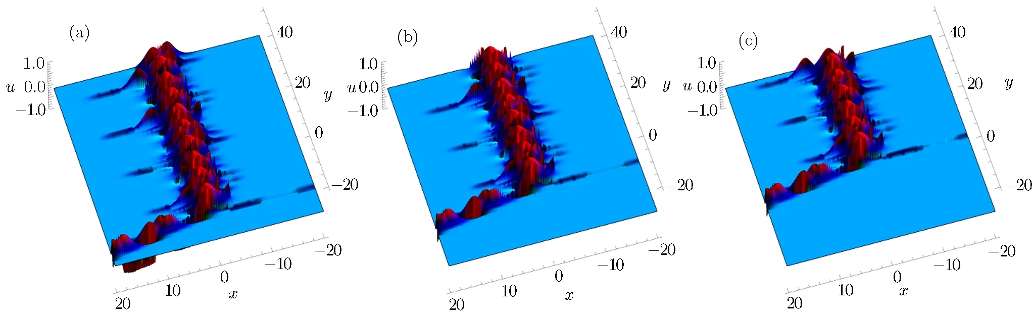
Fig.1 1 The physical structure of solution(61),at α3= β2= α =1,k2=3, γ2= γ3=2,k1= β4= −2,γ1= β1= β3= γ4= −1,(a)t= −10,(b)t=0 and(c)t=10.

Fig.1 2 The physical structure of solution(62),at α3= β2= α =1,k2=3, γ2= γ3=2,k1= β4= −2,γ1= β1= β3= γ4= −1,(a)t= −10,(b)t=0 and(c)t=10.

Fig.1 3 The physical structure of solution(65),at α1= β2= α = ϵ6=1,k1= −2,γ2=2,α3= γ1= β1= γ3= −1,(a)t=−10,(b)t=0 and(c)t=10.

Fig.1 4 The physical structure of solution(66),at α1= β2= α = ϵ6=1,k1= −2,γ2=2,α3= γ1= β1= −1,γ3=0,(a)t= −10,(b)t=0 and(c)t=10.

Case 11

where α,α1,α3,β1,β2,k1,γ1,γ2,and γ3are free real constants,ϵ6= ±1.Substituting these results into Eq.(5),we obtain

Therefore we obtain the eleventh new double-periodic soliton solutions for Eq.(1)as follows:

ξ has been explained in Eq.(64). The evolution and mechanical feature of solutions(65)–(66)are shown in Figs.13–14.

3 Conclusion

In this work,the(2+1)-dimensional breaking soliton equation is investigated.With the help of the bilinear form and the special ans¨atz functions,some entirely new double-periodic soliton solutions for the(2+1)-dimensional breaking soliton equation are presented.All these solutions are brought back to the original equation with the Mathematica software,and the results are all right.Many important and interesting properties for these obtained solutions are revealed with some figures(see Figs.1–14)by the help of symbolic computation software Mathematica.The special ans¨atz functions method is simple and straightforward than the others method.If the bilinear form of nonlinear evolution equations is existent,then rich variety of periodic-soliton solutions can be derived by the special ans¨atz functions method.

[1]K.Hosseini,D.Kumar,M.Kaplan,and E.Yazdani Bejarbaneh,Commun.Theor.Phys.68(2017)761.

[2]W.X.Ma and Y.Zhou,Int.J.Geom.Methods Mod.Phys.13(2016)1650105.

[3]W.X.Ma,J.H.Meng,and M.S.Zhang,Math.Comput.Simulat.127(2016)166.

[4]Z.F.Zeng,J.G.Liu,Y.Jiang,and B.Nie,Fund.Inform.145(2016)207.

[5]S.Ahmad,Ata-ur-Rahman,S.A.Khan,and F.Hadi,Commun.Theor.Phys.68(2017)783.

[6]X.Lü,J.P.Wang,F.H.Lin,and X.W.Zhou,Nonlinear Dyn.,DOI:10.1007/s11071-017-3942-y(2017);X.Lü,W.X.Ma,S.T.Chen,and M.K.Chaudry,Appl.Math.Lett.58(2016)13;X.Lü and F.H.Lin,Commun.Nonlinear.Sci.32(2016)241.

[7]W.X.Ma,Z.Y.Qin,and X.Lü,Nonlinear Dyn.84(2016)923.

[8]M.Eslami,B.F.Vajargah,M.Mirzazadeh,and A.Biswas,Indian.J.Phys.88(2014)177.

[9]X.Lü,S.T.Chen,and W.X.Ma,Nonlinear Dyn.86(2016)1;X.Lü and W.X.Ma,Nonlinear Dyn.85(2016)1217;X.Lü,W.X.Ma,J.Yu,and C.M.Khalique,Commun.Nonlinear.Sci.31(2016)40.

[10]I.Aslan,Appl.Math.Comput.217(2011)6013.

[11]M.Eslami,Appl.Math.Comput.285(2016)141.

[12]F.H.Lin,S.T.Chen,Q.X.Qu,et al.,Appl.Math.Lett.78(2018)112.

[13]M.Eslami,M.Mirzazadeh,and A.Neirameh,Pramana 84(2015)1.

[14]A.Biswas,M.Mirzazadeh,M.Eslami,et al.,Frequenz 68(2014)525.

[15]A.W.Wazwaz,Chaos,Solitons&Fractals 28(2006)1005.

[16]J.G.Liu,Y.Tian,and Z.F.Zeng,AIP Adv.7(2017)105013.

[17]A.M.Wazwaz,Appl.Math.Comput.200(2008)437.

[18]A.M.Wazwaz,Appl.Math.Comput.204(2008)162.

[19]M.Sarker,B.Hosen,M.R.Hossen,and A.A.Mamun,Commun.Theor.Phys.69(2018)107.

[20]A.Qawasmeh and M.Alquran,Appl.Math.Sci.8(2014)2455.

[21]J.G.Liu and Y.He,Nonlinear Dyn.90(2017)363.