Interaction Solutions for Kadomtsev-Petviashvili Equation with Variable Coefficients∗

Jian-Guo Liu (刘建国), Wen-Hui Zhu (朱文慧), and Li Zhou (周丽)

1College of Computer,Jiangxi University of Traditional Chinese Medicine,Jiangxi 330004,China

2Institute of Artificial Intelligence,Nanchang Institute of Science and Technology,Jiangxi 330108,China

Abstract Based on the Hirota’s bilinear form and symbolic computation,the Kadomtsev-Petviashvili equation with variable coefficients is investigated.The lump solutions and interaction solutions between lump solution and a pair of resonance stripe solitons are presented.Their dynamical behaviors are described by some three-dimensional plots and corresponding contour plots.

Key words: Hirota’s bilinear form,dynamical behaviors,stripe solitons

1 Introduction

Nonlinear partial differential equations (NPDEs) are mathematical models to describe nonlinear phenomena in many fields of modern science and engineering,such as physical chemistry and biology,atmospheric space science,etc.[1−6]In recent years,the solutions of NPDEs have become a hot topic,and various methods have been proposed.[6−12]

In these NPDEs,Kadomtsev-Petviashvili (KP) equation can be used to model waves in ferromagnetic media,water waves of long wavelength with weakly non-linear restoring forces and frequency dispersion.[13]However,when modeling various nonlinear phenomena under different physical backgrounds,variable coefficient NPDEs can describe the actual situation more accurately than constant coefficient NPDEs.As an illustration,a KP equation with variable coefficients is considered as follows[14]

whereu=u(x,y,t) is the amplitude of the long wave of two-dimensional fluid domain on varying topography or in turbulent flow over a sloping bottom.The Bäcklund transformation,soliton solutions,Wronskian and Gramian solutions of Eq.(1) have been obtained.[14−16]Lump and interactions solutions have been discussed in Ref.[17].However,interactions among the lump soliton,one stripe soliton,and a pair of stripe solitons have not been investigated,which will become our main task.

The organization of this paper is as follows.Section 2 obtains the lump solutions based on Hirota’s bilinear form and symbolic computation.[18−34]Their dynamical behaviors are described in some plots.Section 3 derives the interaction solutions between lump solution and a pair of resonance stripe solitons.Their dynamical behaviors are also shown in some three-dimensional plots and corresponding contour plots.Section 4 makes a summary.

2 Lump Solutions

Substituting

into Eq.(1),the bilinear form can be obtained as follows

This is equivalent to:

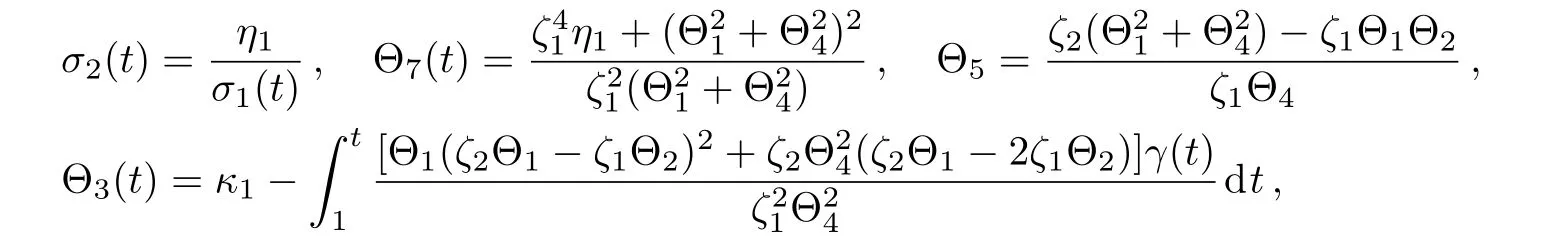
To research the lump solutions,suppose that

where Θi(i=1,2,4,5) are unknown constants.Θ3(t)and Θ6(t)are unkown functions.Substituting Eq.(4)into Eq.(3),we have

with Θ21+Θ24≠0,Θ2Θ4−Θ1Θ5≠0.τi(i=1,2) are integral constants.Substituting Eq.(5) into Eq.(4) and the transformationu=2Θ0[lnξ]xx,the lump solutions for Eq.(1) can be presented as follows

whereξsatisfies constraint condition (5).

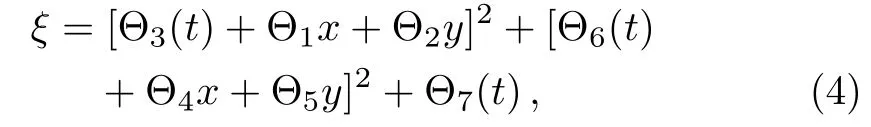
To discuss the dynamical behaviors for solution (6),we suppose that

Substituting Eq.(7) into Eq.(6),three-dimensional plots and corresponding contour plots are presented in Figs.1–3,Figure 1 shows the spatial structure of the bright lump solution on the (y,t) plane,which includes one peak and two valleys.Figure 2 shows the spatial structure of the bright lump solution on the (y,x) plane.Figure 3 shows the spatial structure of the bright lump solution on the(t,x) plane.

Fig.1 (Color online) Lump solution (6) via Eq.(7) when x=0 (a) three-dimensional graph (b) contour graph.

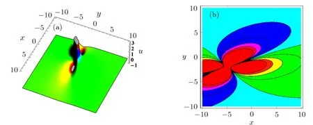
Fig.2 (Color online) Lump solution (6) via Eq.(7) when t=0 (a) three-dimensional graph (b) contour graph.

Fig.3 (Color online) Lump solution (6) via Eq.(7) when y=0 (a) three-dimensional graph (b) contour graph.

3 Interaction Solutions Between Lump Solution and a Pair of Resonance Stripe Solitons

To find the interaction solutions between the lump solution and a pair of resonance stripe solitons,assume that

whereϑi(i=1,2,4,5) andζi(i=1,2) are unknown constants.Θ3(t),Θ6(t),ζ3(t),andσi(t) (i=1,2) are unkown functions.Substituting Eq.(4) into Eq.(3),we have

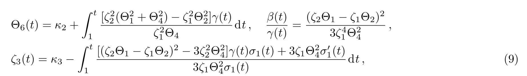
withζ21(Θ21+Θ24) ≠0,Θ4≠0.η1andκi(i=1,2,3) are integral constants.Substituting Eq.(9) into Eq.(8) and the transformationu=2Θ0[lnξ]xx,the interaction solutions between lump solution and two stripe solitons can be presented as follows

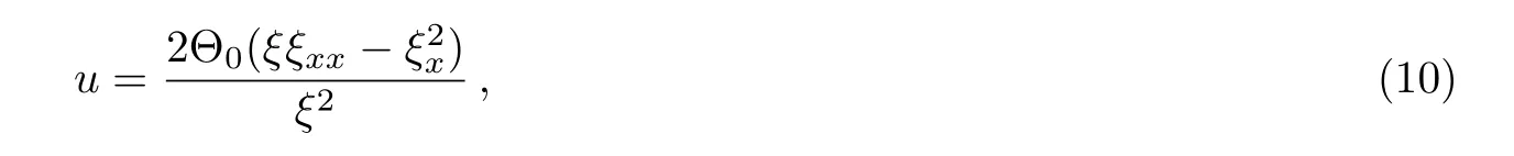
whereξsatisfies constraint condition (9).

To discuss the dynamical behaviors for solution (10),we suppose that

Substituting Eq.(11)into Eq.(10),three-dimensional plots and corresponding contour plots are presented in Figs.4–8.

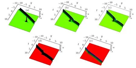
Fig.4 (Color online) Solution (10) via Eq.(11) with γ(t)=1,η1=0 when (a) x=−20,(b) x=−5,(c) x=0,(d) x=5,(e) x=20.

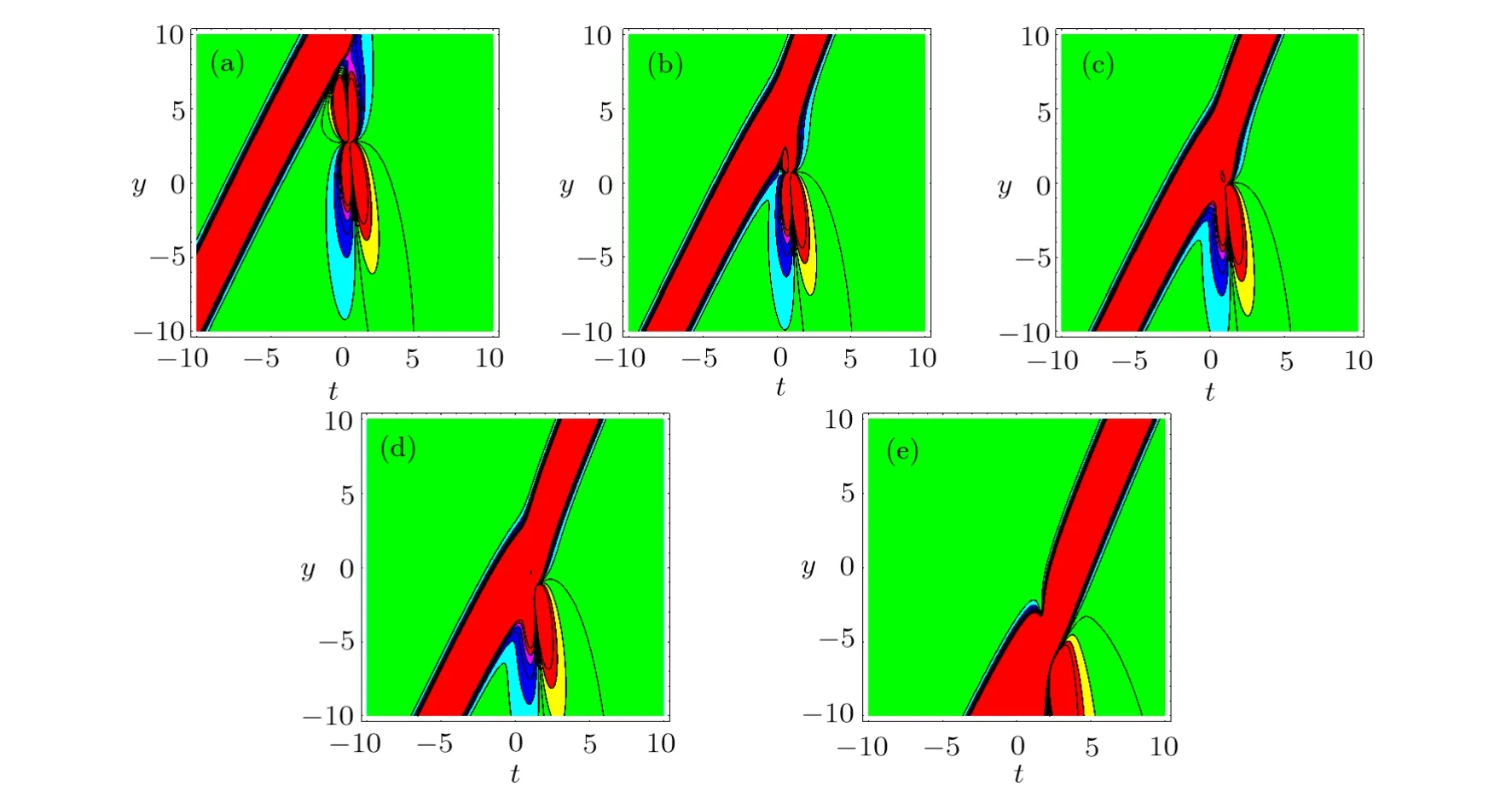
Fig.5 (Color online) The corresponding contour plots of Fig.4.

Whenη1=0,Figs.4 and 5 describe the interaction solution between lump solution and one stripe soliton in the(t,y)-plane,the fusion between the lump soliton and one stripe soliton is shown in Fig.4.Whenx=−20,one lump and one stripe soliton can be found in Fig.4(a).In Fig.4(b),the lump soliton meets with one stripe soliton.In Figs.4(c) and 4(d),we can see the interaction between the lump and one stripe soliton.In Fig.4(e),lump starts to be swallowed until lump blend into one stripe soliton and go on spreading.Figure 5 shows the corresponding contour plots of Fig.4.

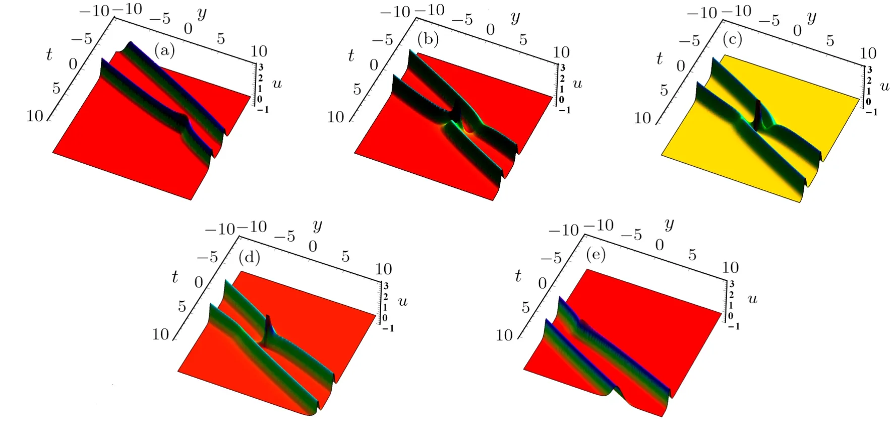
Fig.6 (Color online) Solution (10) via Eq.(11) with γ(t)=1,η1=1 when (a) x=−20,(b) x=−5,(c) x=0,(d) x=5,(e) x=20.

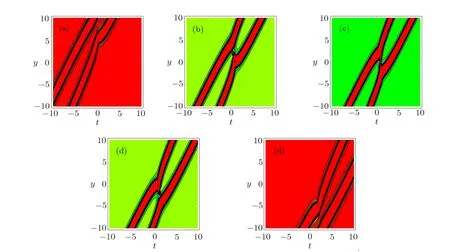
Fig.7 (Color online) The corresponding contour plots of Fig.6.

Whenη1=1,Figs.6,7,and 8 demonstrate the interaction solution between lump solution and a pair of resonance stripe soliton in the (t,y)-plane,the fusion between the lump soliton and two stripe solitons is shown in Fig.6.Whenx=−20,two stripe solitons and one lump can be found in Fig.6(a).In Fig.6(b),the lump soliton meets with two stripe soliton.In Figs.6(c) and 6(d),we can see the interaction between the lump and two stripe solitons.In Fig.6(e),lump starts to be swallowed until lump blend into two stripe solitons and go on spreading.Figure 7 shows the corresponding contour plots of Fig.6 to help us better understand the interaction for solution (10).Figure 8 lists the interaction between the lump and two stripe solitons whenγ(t)=tis a function.

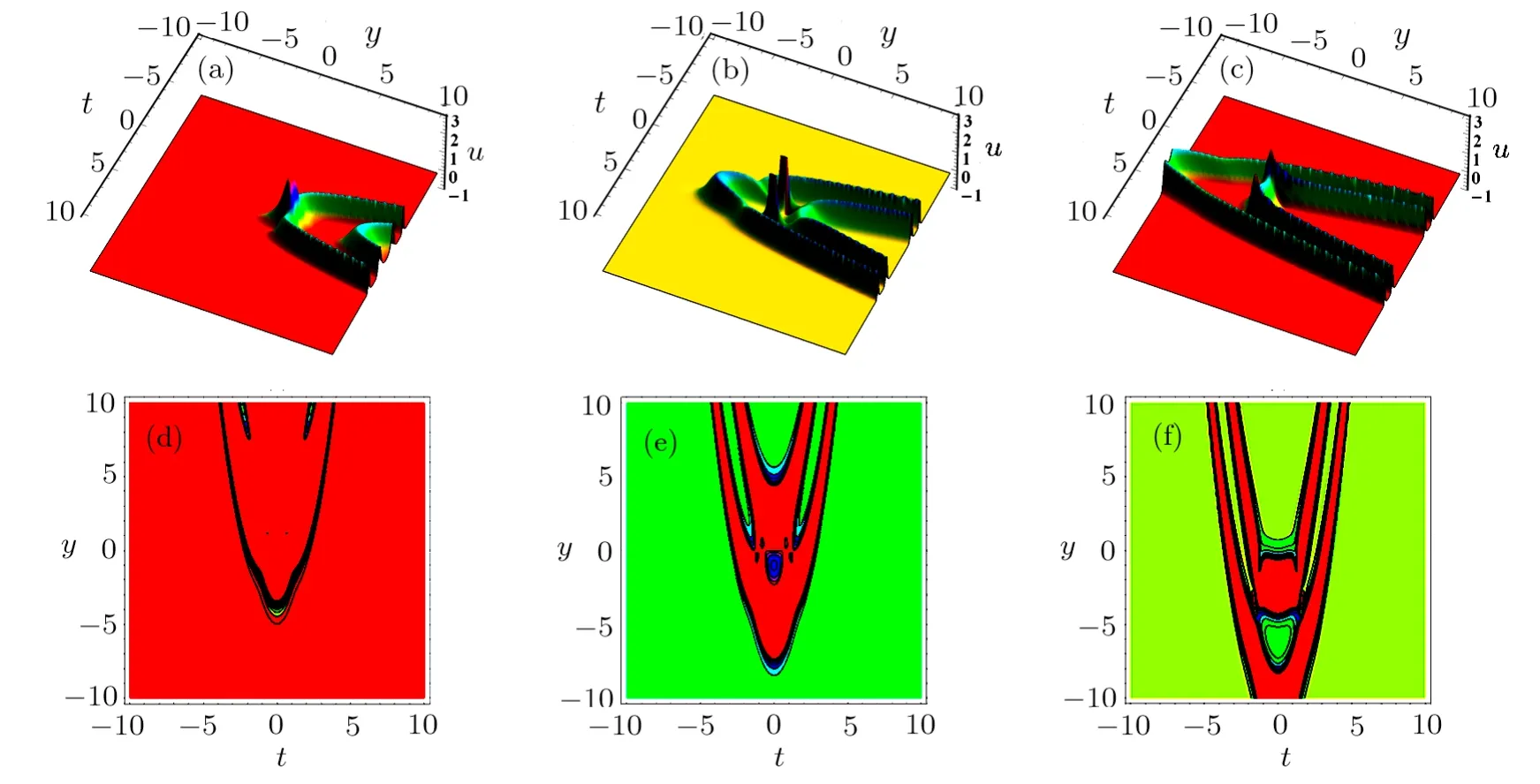
Fig.8 (Color online) Solution (10) via Eq.(11) with γ(t)=t,η1=1 when x=−10 in (a) (d),x=0 in (b) (e),and x=10 in (c) (f).

4 Conclusion

In this work,the (2+1)-dimensional KP equation with variable coefficients are studied based on Hirota’s bilinear form and symbolic computation.Lump solutions and interaction solutions are presented.The spatial structure of the bright lump solution are shown in Figs.1–3.The dynamical behaviors for the interaction solutions between lump solution and one stripe soliton are described in Figs.4 and 5.The dynamical behaviors for the interaction solutions between lump solution and a pair of resonance stripe solitons are shown in Figs.6–8.