Optimal interface surface determination for multi-axis freeform surface machining with both roughing and finishing

Lufeng CHEN,Pengheng HU,Ming LUO,Ki TANG,,*

aHong Kong University of Science and Technology,Hong Kong,China

bNational Numerical Control System Engineering Research Center,Huazhong University of Science and Technology,Wuhan 430074,China

cKey Laboratory of Contemporary Design and Integrated Manufacturing Technology,Ministry of Education,Northwestern Polytechnical University,Xi’an 710072,China

1.Introduction

Multi-axis machining is nowadays widely used in machining freeform surfaces of complicated and high-precision parts,particularly for those large-size parts like blisks of aero-engines and dies and molds in aerospace industry.For a five-axis machine tool,while the two additional rotary axes enable it to possess a larger machining flexibility and achieve a better finish surface quality,its driving ability is often limited due to its complex kinematics and also the relatively poor rigidity of the two rotary tables.On the contrary,in the case of threeaxis machining,as the tool axis remains fixed,the three translational axes can endure much higher velocity,acceleration and jerk during the machining.Based on these different characteristics of the two commonly used multi-axis machining types,to machine a freeform surface out of a raw stock,a two-process strategy is often adopted in practice.In the first process(roughing),a large cutter is used and the machining type is three-axis,with the objective of removing most of the material from the raw stock as quick as possible.In the second process(finishing),a five-axis machine tool is used and the cutter is much smaller;this time the primary objective is to achieve a good finish surface quality and to satisfy the specific machining requirements.

Refer to Fig.1.After the roughing,an intermediate surfaceSris formed so that the volume between the raw stock surfaceS0andSrhas now been removed by means of three-axis machining;this surface will be referred to as the interface surface.After that,in the finishing process,the residual material between this interface surface and the nominal surfaceSfwill be removed by means of five-axis machining.Obviously,with respect to a fixed type of tool path(e.g.,the iso-planar tool path,as adopted in this paper),different interface surfaces will result in different machining parameters(such as the depth of cut)for both roughing and finishing process.Because feed rate assignment on a certain tool path crucially depends on these machining parameters(e.g.,the depth of cut decides the cutting force which in turn directly affects the maximal feed rate allowed),different interface surfaces will lead to different feed rate schedules for both roughing and finishing and consequently result in different amounts of total machining time.

In this paper,we present an implemented optimization algorithm,together with the accompanying physical cutting experimental results,to address this optimal interface surface determination problem:for an arbitrary freeform surfaceSfand a raw stock surfaceS0,given a fixed type of tool path(i.e.,the iso-planar type),the tools for the three-axis roughing and the five-axis finishing,and the two types of most critical constraints on the feed rate–the kinematic capacities of the machine tool and the maximum deflection cutting force on the cutter,our algorithm aims at finding the best interface surfaceSrso that the total machining time of the resultant roughing and finishing process will be minimized.As convincingly confirmed by our physical cutting experiments,such an optimal interface surface often substantially improves the machining efficiency compared with the traditional offset surface.

This paper is organized as follows.In Section 2,a review on the background of this research is given.In Section 3,the isoplanar tool path generation scheme is introduced,and followed by a detailed description of how the in-process workpiece(IPW)is efficiently calculated in the machining process,which determines the cutting force.In Section 4,the optimal feed rate scheduling strategy is given,which considers both the kinematical constraints of the machine tool and the specified de flection cutting force threshold.In Section 5,the construction and optimization algorithm for the interface surface is presented,which is followed by the experimental results and the discussion in Section 6.The paper is concluded in Section 7.

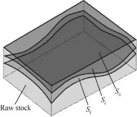
Fig.1 Illustration of machining stock.

2.Literature review

In the existing works of multi-axis machining of freeform surfaces,much effort has been spent on improving the machining efficiency.In general,they mainly focus on two aspects:one is to reduce the total tool path length with regard to the workpiece itself,and the other is to optimize feed rate for an already generated tool path,so that the tool can move at a higher speed subject to certain physical constraints(such as the maximum cutting force and/or the kinematical limits of the machine tool).

Currently,the most popular types of tool paths in multiaxis machining of freeform surfaces are iso-parametric1–3,iso-planar4–7, and iso-scallop height.8–10For the isoparametric and iso-planar type,they inevitably suffer from a common problem of machining redundancy between the cutter contact(CC)curves;in other words,the total length of the tool path is not minimized.Targeting at this issue,the iso-scallop height method as proposed by Suresh and Yang8tried to eliminate CC curve redundancy by maintaining a constant scallop height between the neighboring CC curves,and the total tool path length could be reduced in this way.Following this idea,there is a large number of works aiming at further reducing the total tool path length such as by selecting an optimal master cutter path(MCP).11–14Nevertheless,in all these works(Refs.8–14),the tool path is generated in the workpiece coordinate system(WCS),independent of the specific machine tool on which the final physical machining will be executed,and,as always,a constant feed rate is assumed.As a consequence,the machining efficiency is typically not really optimized since the machine tool often has to work at a relatively low feed rate lest its kinematical constraints are violated.

There are also studies on machining efficiency with the kinematical constraints of the machine tool considered.Kim and Sarma15introduced a vector field by taking the drives’speed limits into consideration to generate the so called timeoptimal MCP.Aimed at maximizing the kinematical performance of the machine tool,Sencer et al.16developed a feed rate scheduling algorithm for the real time control of the computer numerical control(CNC)systems by assigning the optimal feed rate without violating the five drives’kinematical constraints.To further reduce the machining time,Beudaert et al.17identified and smoothed the critical points on the CC curves that limit the motions on the joints.Sun et al.18proposed a novel method and used a curve evolution strategy to smooth the feed rate profile for NURBS tool paths by changing the positions of those CC points which violate the kinematical constraints.By combining the cutting strip width and the kinematical performance,Hu and Tang19proposed a vector field called Machine-Dependent Potential Field(MDPF)as well as a tool path generation scheme which tries to align the feed direction with the principal MDPF direction everywhere on the surface.

In addition to the kinematical constraints of the machine tool,there are also other types of physical constraints on the feed rate,among which the particularly critical one is the deflection cutting force on the cutter–large deflection cutting force will cause the cutter to bend,shorten its service life,and seriously jeopardize the quality and accuracy of the finished surface.The first cutting force model for ball-end milling was developed by Lee and Altintas20,and followed by a variety of studies focusing on predicting the instantaneous cutting forces in the area of different cutter profiles21,22and cutting force models.22–24As a precise prediction on the cutting force crucially depends on the correct calculation of the instantaneous cutter-workpiece engagement(CWE)region,people also looked into the tool engagement analysis.Kim et al.25first used the Z-buffer method to estimate the cutter contact area in three-axis ball-end milling;Zhu et al.26and Fussell et al.27then extended theZ-buffer updating strategy to multi-axis ball-end milling.The predicted cutting force can be used to improve the machining efficiency.To further accurately predict the cutting force in multi-axis machining,Sun and Guo28and Li et al.29extended the classical cutting force model and proposed the method to calculate the CWE accurately considering the cutter runout effect.Kurt and Bagci30thoroughly reviewed and compared the feed rate optimization algorithms based on the material removal rate(MRR)with those based on the cutting-force,and found that the latter provide significant advantages due to its accuracy.Zeroudi and Fontaine31used the cutter deflection model32to predict the deflection force analytically,while Xu and Tang33numerically calculated the maximum deflection force based on the cutting force model introduced by Engin and Altintas22,which in turn limits the maximum feed rate since the cutting force is approximately linearly proportional to the feed rate.

For all the aforementioned works,they exclusively focus on the finishing process with a simple assumption that the interface surface is an offset from the nominal surface,thus ignoring the effect of its actual shape which in general is not a simple offset of the nominal surface.As a result,the calculation of material removal volume and CWE are not accurate.Consequently,the corresponding cutting force models cannot reflect the real situation of machining an arbitrary interface surface.

Compared to the finishing process,it is the roughing process(including semi-finishing process)that typically takes over the majority of the material removal job.Normally,the roughing process for a freeform surface is made of layer-by-layer 2D pocket milling,and the total machining time depends on the 2D milling tool path pattern and the number of layers.For layer-by-layer milling,zigzag pattern of tool path is commonly used owing to its simplicity compared to the contour method.34However,because of the lack of the mechanistic knowledge of both the workpiece and cutter,the constant depth of cut is always chosen empirically and conservatively to prevent tool breakage and chatter.Under such a simple scheme,if the part is curvy and has many peaks and valleys,many intermediate islands would emerge during the machining which the tool has to air-move over,thus wasting time in non-cutting transits.Another drawback of 2D pocketing is that the stair-case like residue left after the process may lead to sharply changing chip load in the following cutting,which in turn may jeopardize the surface quality and increase the tool wear.To resolve the problem,some studies have focused on finding more efficient and robust tool path patterns in roughing with variable depth of cut.Lefebvre and Lauwers35introduced the morphing techniques in finding a smooth intermediate geometry to avoid the stairs-like shape geometry left by the roughing in threeaxis machining.They also used five-axis instead of three-axis machining for the roughing in order to achieve a better surface finish quality.However,their methods failed to indicate the total machining time,and no comparison between theirs and the traditional ways was given.Xu and Tang36extended the idea to formulate the tool path planning strategy for roughing using three-axis ball-end cutter with the attempt to save total energy usage during the machining.After roughing and finishing,the entire machining process typically ends up with a clean-up operation to remove the uncut volume left.37

3.Modeling and updating of in-process workpiece

Given a certain interface surface,the volume to be removed in the raw stock can be divided into two parts,i.e.,the ones to be removed by roughing and those by finishing.In the process of machining along a certain tool path,the volume of the workpiece keeps changing,where the sweeping of the tool on the surface keeps removing the material from the workpiece.Such kind of workpiece whose volume is constantly updated is naturally called an in-process workpiece(IPW).For a given tool path,in order to assign the maximally allowed feed rate at each cutter location,its loading(i.e.,both kinematical and mechanical load)should be precisely calculated,which in turn requires a precise modeling and accurate estimation of the IPW.

In this paper,one of the most popular types of tool path,the iso-planar type,is chosen for both roughing and finishing.To clearly explain our idea,the iso-planar tool path generation is first briefly introduced,based on which the method of precise and efficient estimation of IPW is then presented.

3.1.Iso-planar tool path generation

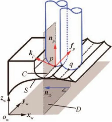
Fig.2 Iso-planar tool path generation.

For a three-axis roughing operation,since the tool axis is fixed,the CC curves alone are sufficient to define the tool path to machine the interface surface.However,for a five-axis finishing operation,in addition to the generated CC curves,variable tool orientation should also be determined for them.In this paper,a fixed local tool orientation is chosen in the LCS at each CC point,i.e.,wp= ［α,β］= ［10°,0°］(that is,the tilt angle α =10°and the yaw angle β =0°).Refer to Fig.3(a),given a CC curveCand the corresponding tool orientation wp,the multi-axis tool path alongCcan be represented as a series of pairs （pt,wp）,whereptis the cutter location(CL)point and wpits associated tool orientation in WCS.For details about the determination of tool orientation and the relationship between the CC point and the CL point,please refer to Ref.38.With the tool path generated,the IPW can be precisely estimated,as to be elaborated next.

3.2.Updating strategy for in-process workpiece

As the tool cuts the surface by sweeping along a pre-defined CC curve,the geometry of the(changing)IPW should be updated accordingly.Fig.4 shows an instantaneous cutting case with the cutter immersing into the workpiece(represented as a polyhedron)between the raw stock surfaceST0and the nominal surfaceST,both in triangulation form.

wherev∈ ［0,1］,sT= （x,y,z）andsT0= （x0,y0,z0）are the corresponding nodal positions onSTandST0respectively.

Fig.3 Illustration of a five-axis tool path and parametric representation of a ball-end cutter.

Fig.4 Definition of in-process workpiece.

In a typical calculation of the removed volume in machining,except for the very first CC curve,when the cutter moves along the current CC curveC,it is actually not fully submerged in the volume betweenST0andST,since the previous cuts will have already left ‘grooves” onST.As this pregroove effect is significant(since adjacent CC curves are very close to each other),it must be considered so that the cutting force can be accurately calculated.33

In our setting,this pre-groove effect can be recorded by updating the ZDVs ofSTin accordance with the cutter’s movement along a CC curveC,which can be achieved by calculating the intersection between each ZDV and the cutter movement envelope generated alongC.For a ball-end cutter moving on a CC curve as shown in Fig.3(b),it can be parametrized following two trajectories:CC curve and tool axis parametrized bytandsrespectively,i.e.,

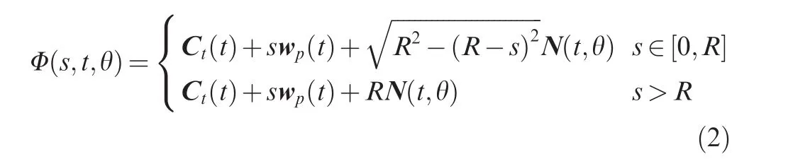
where θ ∈ ［0,2π）andt∈ ［0,1］,Ct（t）represents the trajectory of tool tip along a CC curveCformed by a serial of CL pointspt（t）,Ris the tool radius,and the casess∈ ［0,R］ands＞Rrepresent the semi-spherical part and the cylindrical part of the cutter respectively.A tool coordinate system (TCS)up-vp-wpis defined at CC pointpwith wprepresenting the tool axis.Note that it is only a function of parametertalong the CC curve.N（t,θ）is the normal vector perpendicular to wp（t）,which determines the characteristic circle of the revolute surface that represents the cutter,i.e.,

As consecutive CC points on the CC curve are very close to each other,we assume that the cutter moves linearly from one CC point to its successor without tool orientation change.It should,however,be noted that this simplification is only an approximation in modeling the swept envelope of a multiaxis tool path.To increase its approximation accuracy,the resampling strategy of the tool path is performed under two criteria:(1)the spacing between every pair of neighboring CC points is constrained by chord error δ1;(2)the angle between two neighboring orientation vectors is constrained by an angular error δ2.In another word,if the CC curve propagation fails in either condition,the next CC point is replaced by a closer one(such as the middle point).Fig.5 shows the swept envelope generated by moving the cutter from CC pointptoqalong the instantaneous feed direction fp,which is determined by three parts:

where Φp（s,t,θ）is the ingress point set at pointpwith N（t,θ）·fp＞ 0,Φq（s,t,θ）is the egress point set at pointqwith N（t,θ）·fp＜ 0,and for Φ0（s,t,θ）,the grazing point set has the following relationship:

Based on Eq.(7),the condition for the grazing point can be solved as

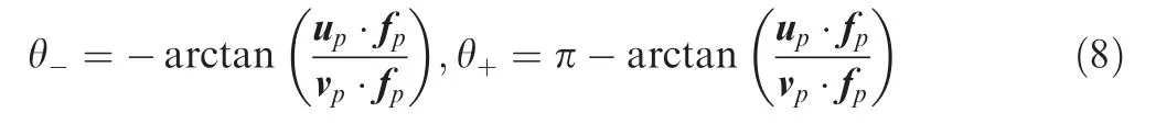
where θ-and θ+are the two solutions for θ (as defined in Eq.(2)),which define the corresponding grazing curve on the surface of the cutter for a particulart.By substituting Eq.(8)into Eq.(7),the solution for the grazing point set on Φ0is obtained.

From the above analysis,to find the intersections between ZDVs and the swept envelopeE,each ZDV is tested againstEby combining Eq.(1)with Eq.(8):

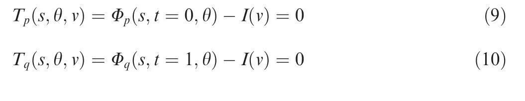
Fig.5 Geometric description of swept envelope generated from CC point p to q.

For each of Eqs.(9)–(11),it is a nonlinear function with three variables,and the number of constraints for each function is also three.Thevvalue from the solutions of Eqs.(9)–(11)can be used to update the ZDV defined in Eq.(1).

The intersections in Eqs.(9)and(10)can be determined in a similar way,except that this time by substituting the equivalent ofsfromTxp（s,θ）=0(orTxq（s,θ）=0)intoTyp（s,θ）=0(orTyq（s,θ）=0)a nonlinear equation about θ is obtained.Instead of solving it explicitly,we treat the intersection as a linecylinder(or line-sphere)intersection problem.Fig.5 shows an example of ZDVs intersecting a cutter.Specifically,the intersection between a lineIexpressed by Eq.(1)and a cylinder located atOp(orOqwhen the cutter contacts CC pointq)with direction vector wpcan be solved by

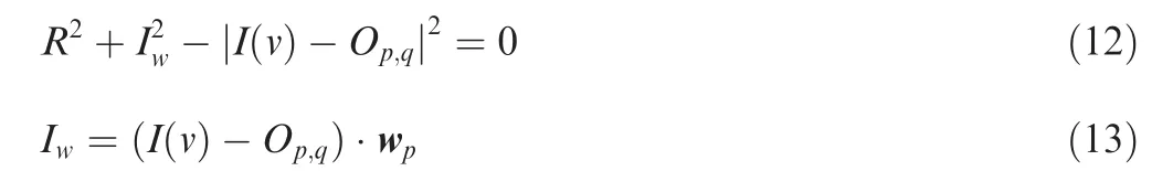
whereIwis the length between the intersection point and the cutter’s center projected onto wp,I（v）a point on lineIandRthe tool radius.As for the intersection between a lineIand a sphere located atOp(orOq)with radiusR,the following equation is in order:

By solving the above two quadratic equations,the value of parametervis obtained,which can be used to determine whether the corresponding ZDV should be updated or not during the machining process when the cutter sweeps on surfaceST.

Note that there could be multiple solutions forvfrom Eqs.(9)–(14),and the final one taken for the ZDV updating should be:

wherevp,vqandv0are the correspondingvvalues solved for the three cases in Eq.(6).Note that for allvp,vqandv0themselves,there could also be multiple values.

With the pre-grooving effect efficiently taken care of by updating ZDVs,the IPW can now be quickly and accurately determined.The entire process can be outlined by the following procedure.

Step 1:Represent the IPW by a simplified vector model with the triangulated nominal surface STand a set of correspondingz-direction vectors ZDVs defined at the nodes of STwith their lengths representing the depths between the raw surface ST0and ST.

Step 2:For the current CC curve,calculate thezvalue by finding the intersections between ZDVs and the swept envelope E generated by the tool motion.

Step 3:Update thezvalue in the IPW according to thezvalue obtained in Step 2.

Step 4:Repeat Step 2 and Step 3 for the next CC curve until the entire tool path is processed.

Fig.6(a)depicts a ZDV updating example.The initial raw surfaceST0is a plane,and some portion of the workpiece has already been machined by the previous CC curves.The tool orientations at some CC points at the current CC curve are also shown.In step 2,traditionally,thezvalue of ZDVs is updated by intersecting all the ZDVs with the generated swept envelope using Eqs.(9)–(14),which is very time consuming.To improve the computational efficiency,after one CC curve is generated by plane&mesh intersection,a list of potential ZDVs are filtered out to form a local polyhedron whose distance to the current cutter location is within a preset range(2Ris used in the example).Then effective cutting edge can then be calculated quickly in this local polyhedron.

Fig.6(b)shows a comparison of two local polyhedrons with and without the pre-grooving effect.In Fig.6(b1),the instantaneous local polyhedron is built by the ZDVs that are updated in accordance with the previous CC curve(s),while the one in Fig.6(b2)considers only the ZDVs associated with the current CC curve.As pointed out by Xu and Tang33,the corresponding mean deflection force could differ by as much as 40%with and without the pre-grooving effect.

4.Optimal machine-dependent feed rate scheduling

In multi-axis machining,once the tool path is determined,the only factor left which can affect the machining efficiency is the feed rate,which is limited by the physical constraints of the specific machine tool.In general,among others,there are two major types of constraints on the feed rate–the kinematical constraints and the cutting force constraint.Let us first analyze the relationships between the feed rate and these two physical constraints and then present our optimal feed rate scheduling method based on these relationships.

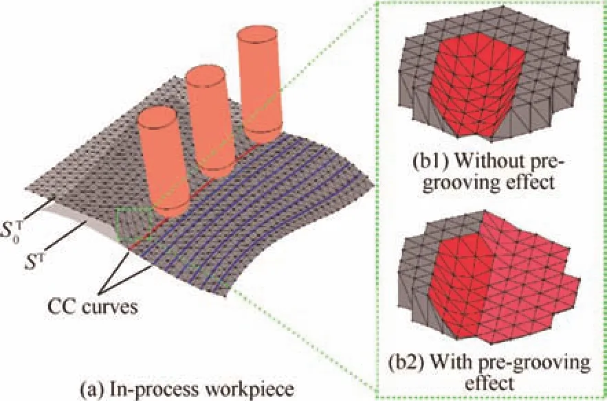
Fig.6 Illustration of in-process workpiece in five-axis machining.

4.1.Kinematical constraints on feed rate

For a certain machine tool,its kinematic capacities are defined as the maximal allowable velocity,acceleration,and jerk of the machine’s all axes(three axes for three-axis machining and five axes for five-axis machining).As already alluded,when machining a freeform surface such as a die or mold,typically three-axis machining is adopted for the roughing process so that most of the material can be removed from the raw stock at a much higher feed rate,while five-axis machining is employed for the final finish cutting(and semi-finish cuttings if needed)to achieve a higher surface finish quality,but with a much slower feed rate due to the relatively weaker kinematic capacities of the two rotary axes.

On one hand,the kinematic capacities are defined with respect to the machine coordinate system(MCS);on the other hand,the tool path is defined in WCS.To relate the two with each other,we need first to establish the relationship between them.

Given a five-axis tool path(including both the CL curve(s)and the associated tool orientation),after the Inverse Kinematic Transformation (IKT),it becomes a five-tuple M= ［x,y,z,B,C］corresponding to the coordinates of thexyzlinear axes and the B and C rotary tables(without loss of generality,we will use B-C table-tilt type five-axis machine tool as the illustrative example).In order to numerically get the velocity,acceleration and jerk of a CC pointpin MCS,four more neighboring points （p-2,p-1,p1,p2）are needed on the CC curve,with a small sample distancel,as shown in Fig.7,from which their corresponding IKT results（M-2,M-1,M,M1,M2）can be calculated(refer to Ref.19)and the velocities,accelerations and jerks of the axes can be numerically approximated as

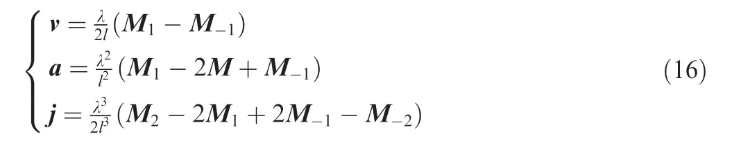
where v,a and j are the velocities,accelerations and jerks of machine’s five drives,while λ is the feed rate.

Note that in Eq.(16),the sample distancelshould be sufficiently small so that the feed rate λ can be assumed to be the same in a small neighboring range ofp.

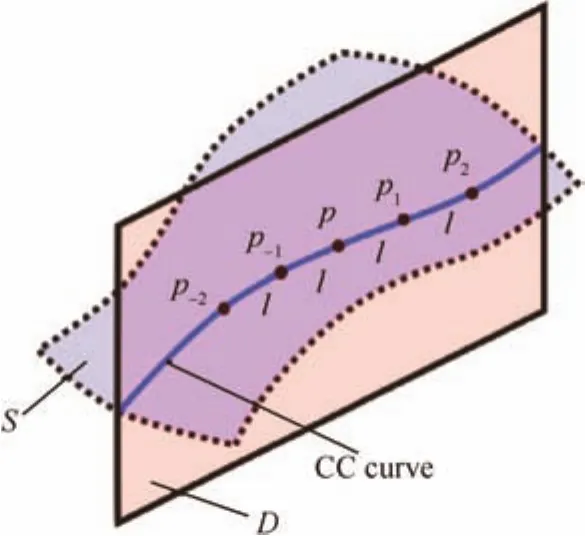
Fig.7 A CC point p with its four neighboring sample points on one CC curve.

For any five-axis machine tool such as the one shown in Fig.8,there are kinematical constraints on all its five axes:

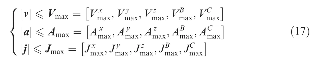
where Vmax,Amaxand Jmaxare respectively the maximally allowed velocities,accelerations and jerks of the machine’s five drives,and they will be referred to as the kinematic capacities of the machine.

By substituting Eq.(17)into Eq.(16),the estimated feed rate at CC pointpshould be capped as

The maximally allowed feed rate atpunder the above kinematical constraints,denoted as λk,should then be the one subject to the most stringent constraint of the totally 15 constraints,i.e.,

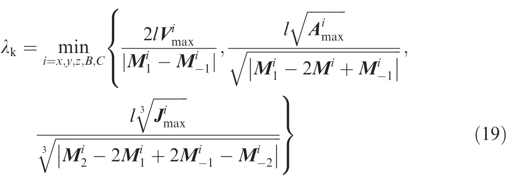
By applying Eqs.(16)–(19)to each CC point,the maximally allowed feed rate for every CC point can then be determined.

The above process of obtaining the maximally allowed feed rate is for a general five-axis machine tool;as for a three-axis one,the treatment is simpler–in Eq.(19)only thexyzaxes need to be considered.

With the above Eq.(19)dealing with the kinematical constraints of the machine tool,we now move to another important constraint on the feed rate–the cutting force constraint.

4.2.Cutting force constraint on feed rate

In multi-axis machining,to protect the cutter and also ensure a good machining accuracy,the deflection cutting forceFdon the cutter should be controlled,i.e.,it should never exceed a certain thresholdFd0,defined as the maximally allowed deflection force.There are of course other types of cutting force related constraints,e.g.,when machining a thin-walled workpiece,the bending of the workpiece due to the cutting force becomes a major concern.Nevertheless,in this paper,we will focus exclusively on the deflection cutting force on the cutter,understanding that the analysis and methodology proposed here can be easily adapted to other types of cutting force related constraints.

For the sake of self-completeness,let us briefly review the classical cutting force calculation model proposed by Engin and Altintas22,which is adopted by us.According to Ref.22,the cutting force components on one flute acting on a moving cutter in the tool coordinate system(TCS) （u-v-w）are given as follows:

whereFu,FvandFware the total cutting forces in u,v and w directions in the TCS respectively,and dFu,dFvand dFwthe differential cutting forces acting on a differential portion of the effective cutting edge segment in TCS between the entry pointPentand the exit pointPexton a flute,which is determined by the IPW as already described in Section 3.2 and the feed rate.

Fig.9(a)shows an instantaneous cutting state with the cutter immersing into the IPW(represented as a polyhedron)between the raw stock surfaceST0and the nominal surfaceST,both in triangulation form,wherehcis the cutting length.As indicated by Eq.(20),the total cutting forces are solely determined by the effective cutting edge(ECE)segment ECE=PentPextwhen the tool orientation and feed rate are fixed.Instead of trying to de fine ECE analytically,the discrete approach is usually adopted,i.e.,the cutting edge on the cutter is uniformly sampled into a discrete point setPc= ｛P1,P2,...,Pi,...｝.The point containment test is then performed to decide whetherPiis inside the IPW or not.As the shape of IPW strongly affects the result of point containment test,different shapes of IPW will have different effective cutting edge segments ECE,and thus different cutting forces.

Fig.9 Cutting force model.

The infinitesimal cutting force components （dFt,dFr,dFa）at a validPion ECE is calculated as

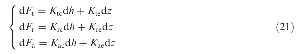
whereKtc,KrcandKacare the shear force coefficients on tangential,radical and axial direction respectively,andKte,KreandKaethe edge cutting coefficients on tangential,radical and axial direction respectively.These 6 coefficients are constants that are usually calibrated with experiments,and dhand dzare the differential chip load and differential projected cutting edge onto the tool axis respectively.

Note that the infinitesimal cutting force components in Eq.(21)are evaluated in terms of the local edge geometry;for integration purpose,they should be converted to the global TCS by a transformation matrix MTLthat is determined by the immersion angle and the spindle rotation angle atPi.For details about the transformation matrix,please refer to Ref.33.Then,the differential cutting forces become

By using Eq.(20)to sum up all the differential cutting forces on the valid cutting points on the effective cutting edge,the instantaneous cutting force is obtained.As the deflection force acting on the cutter is perpendicular to its axis w,its magnitude becomes

AsK（θ）varies with θ,letKmax=max｛K（θ）:θ ∈ ［0,2π］｝ (in our implementation,this is achieved by sampling ［0,2π］intokangles Θ = ｛θ1,θ2,...,θk｝and then calculating eachK（θi）).The maximally allowed feed rate λmat CC pointpwith respect to the specified deflection force thresholdFd0is then defined as

4.3.Feed rate scheduling strategy

With respect to a given tool path,for any CC pointpon it,the maximally allowed feed rate forpis then the smallest of the three thresholds:

where λkand λmare decided by Eqs.(19)and(25)respectively,while the third one λpis a user-defined absolute maximum for the feed rate.

By applying Eq.(26)to each CC point,we can generate the feed rate profile λ*（s）along the CC curve-basically it is the lower envelope of the three functions λk（s）, λm（s）and λp（s）(sbeing the arc length of the CC curve).Fig.10 shows an illustrative example of λ*（s）along a CC curve,and the green colored curve is the maximally allowed feed rate profile.From the figure,we can find that curve is onlyC0.As suggested by Ref.17,the feed rate profile is preferred to be at leastC2in order to avoid slowdown of the machine tool.Therefore,in this work,we smooth the feed rate profile by the classical B-spline interpolation method.If better smooth quality is needed,more details can be found in Ref.17.

5.Determination of optimal interface surface

Refer to Fig.11.Given a block of raw materials with the raw surfaceS0and the final surfaceSf,the toolUr(with a larger radius)for the three-axis roughing process,and the toolUf(with a smaller radius)for the five-axis finishing process,our task is to find an ‘optimal” interface surfaceSrin the block betweenS0andSf,which separates the roughing process from the finishing process.The criterion for the optimum ofSris exactly the machining efficiency,i.e.,with the scallop-height threshold on the final machined surface upheld,we want to minimize the total machining time counting both roughing and finishing processes and subjected to the maximally allowed feed rate λ*(Eq.(26)).Traditionally,Sris simply an offset surface ofSfwith a small offset distance,and to ensure the final finishing surface quality,a very conservative(usually constant)feed rate is adopted for the finishing cutting.As to be seen from the results of our experiments,such an overly simplified approach often severely underutilizes the resources and ends up in an unnecessarily long total machining time.

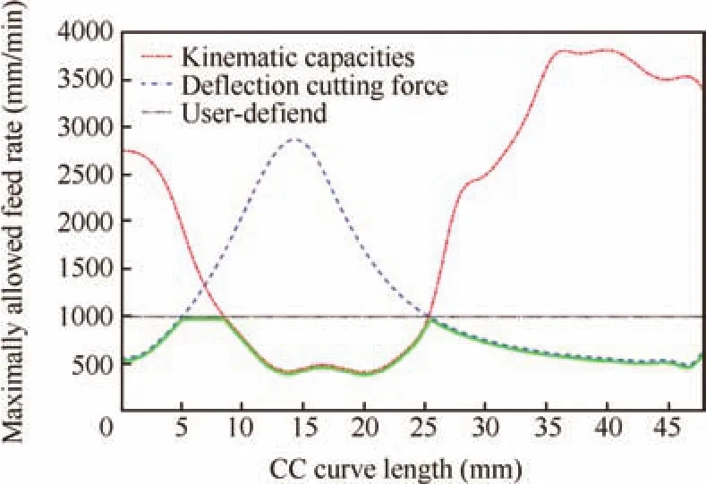
Fig.10 Maximally allowed feed rate λ*along a CC curve under three constraints λk,λmand λp.

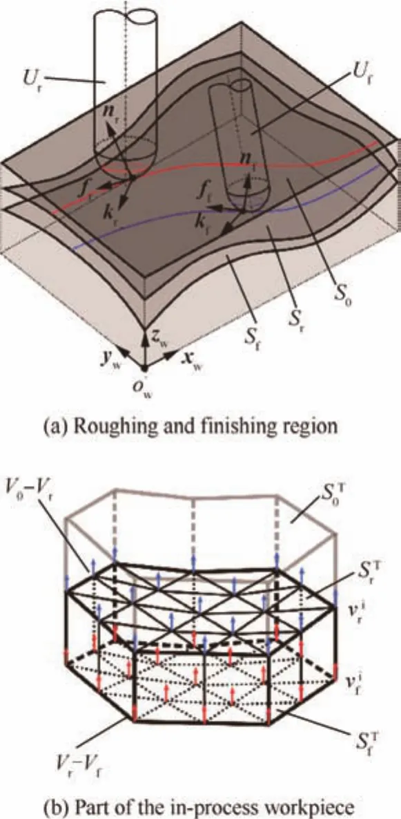
Fig.11 Illustration of machining regions.

5.1.Modeling of interface surface

In our approach,the interface surfaceSris modeled as a B-spline surface with （m+1）× （n+1） control points CP= ｛P00,P01,...,Pmn｝:

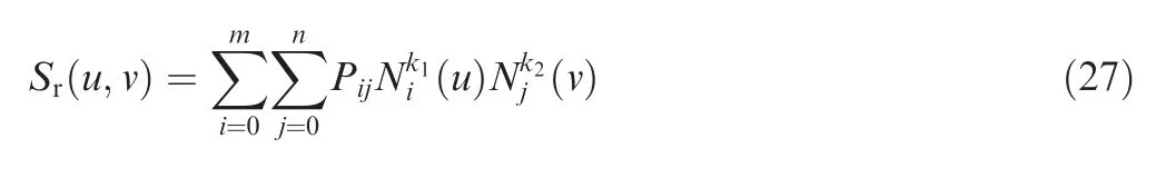
ForSr（u,v）in Eq.(27),its smoothness is determined by degreek1andk2,while its shape is controlled by the number and the distribution of the control points.In order to precisely represent the interface surface as an arbitrary surface,more control points are preferred.On the other hand,too many control points would make the problem too computationally complicated.Details for the selection and distribution of the control points will be introduced in Section 6.

The raw surfaceS0,the interface surfaceSr（u,v）,and the nominal surfaceSfare all discretized into their respective triangulated mesh formST0,STrandSTfwith their respective node setsV0= ｛v10,v20,...,vn0｝,Vr= ｛v1r,v2r,...,vnr｝ andVf= ｛v1f,v2f,...,vnf｝.For the convenience of representation and update of the IPW,the nodes inV0andVrwill share the samex-andy-coordinates with those inVfand the three will also have the same triangulation topology.In this case,the volume betweenS0andSfcan be represented by two sets of discrete vectors in thezdirection passing through the node setsV0,VrandVf–those betweenV0andVr,i.e.,V0-Vr(e.g.,the blue colored in Fig.11(b)),and those betweenVrandVf,i.e.,Vr-Vf(e.g.,the red colored in Fig.11(b)).

5.2.Optimization of interface surface

For both roughing and finishing process,iso-planar tool paths can be generated,i.e.,a three-axis tool path for rough cuttingSrand a five-axis tool path for finish cuttingSf,where the machining parameters for these two processes,i.e.,the cutter radius and the specified scallop-height,are different.

For a generated tool path,either roughing or finishing,the feed rate for each CC point will be assigned according to Eq.(26),and the total machining time can then be approximated as

whereNis the number of CC curves,mithe number of sampled CC points on thei-th CC curveCi,andpi,jthej-th CC point on thei-thCiwith feed rate λ*i,j(calculated from Eq.(26)).

From Eq.(28),both the machining timetrfor roughing andtffor finishing can be found,and the total machining timeFtfor the entire machining process then becomes

As the tool path generation strategy is predetermined(refer to Section 3.1)and the feed rate scheduling is also automatically determined according to Eq.(26),the only variable left to influence the total machining timeFtis the interface surfaceSr,whose control variables are its control points.On one hand,the shape ofSraffects the depths of cut of both roughing and finishing,which in turn affect the maximally allowed feed rate λ*i,jin Eq.(28).On the other hand,sinceSrwill act as the finish surface for the roughing tool path,it has direct influence on how the roughing tool path will be generated.The final task then is to determine the optimal positions of the control points CP so that the total machining timeFtcan be minimized.

This is a high-dimensional and highly nonlinear minimization problem–even for a simple B-spline surface with only 3×3 control points,there will be totally 27 variables to optimize.To simplify it,we capitalize on the fact that in our setting the volume betweenS0andSris modeled as a height field(in thezdirection).In such a case,only thez-values of the control points need to be optimized.Specifically,the （m+1）× （n+1）control points are first evenly distributed on theowxwywplane,i.e.,CPx= ｛x00,x01,...,xmn｝ and CPy= ｛y00,y01,...,ymn｝with the degreek1andk2fixed;the B-spline surfaceSr（u,v）is then determined only by changing thez-values of the control points,i.e.,CPz= ｛z00,z01,...,zmn｝.Measure which is taken in this way not only tremendously decreases the number of variables(by 2/3)but also makes the control of the shape ofSrmore manageable.As the result,the final optimization problem becomes

wherez0（xij,yij）andzf（xij,yij）are the correspondingzcoordinates ofS0andSfrespectively given thex-andycoordinates （xij,yij）,and δland δuthe safety tolerances in case there is some air cutting in the roughing or finishing process.

The optimization problem of Eq.(30)has（m+1）× （n+1）variables,which can be solved by either a standard nonlinear optimization algorithm(e.g.,the interior point method)or some heuristic-based optimization methods(e.g.,the Genetic Algorithm).In our work,the interior point method solver in MATLAB is used to solve Eq.(30).

6.Experiments and discussion

We have implemented our entire interface surface optimization algorithm in MATLAB,namely theTime-Efficient-Total-Machiningsoftware.While the Interior Point Method Solver in MATLAB is called as a subroutine in the computer program to solve the formulated optimization problem of Eq. (30), the procedural function evaluationFt（z00,z01,...,zmn）itself,which includes iso-planar tool path generation for both roughing and finishing and the calculation of Eq.(26),is completely carried out by our own codes.In this section,we report the experimental results of softwareTime-Efficient-Total-Machiningon two freeform test surfaces in both computer simulation and physical cutting.The results are also compared with those of the traditional simple offset surface method,and the comparison data convincingly validates the motivation behind the proposed work.

The first test surfaceSfis shown in Fig.12,which is defined over a regular square in thexyplane with a dimension of 50 mm×50 mm.The raw surfaceS0(not shown in the figure)is a flat face parallel to thexyplane and 0.5 mm above the highest point onSf.

The experimental setting for the test is as follows:two ballend cutters(i.e.,UrandUf)with radiusRr=3 mm andRf=2 mm are chosen for the roughing and finishing processes respectively;the scallop-heighthfor both finishing and roughing is 0.1 mm;the maximally allowed deflection forces are 500 N(for roughing with cutterUr)and 300 N(for finishing with cutterUf);the spindle speed is 8000 r/min;the shear force coefficients are calibrated asKrc=928 N/mm2,Ktc=724 N/mm2,andKac=196 N/mm2,while the edge coefficients are calibrated asKre=20 N/mm,Kte=70 N/mm,andKae=2 N/mm.

The five-axis machine tool JD-GR200_A10H is chosen as the platform to conduct the physical cutting experiment,which is of table-tilt orthogonal B-C type(as shown in Fig.8)with the following manufacturer suggested kinematic capacities:

where the first three columns are the kinematic capacities of the three translational axes in velocity(mm/s),acceleration(mm/s2)and jerk(mm/s3),and the last two ones are for the two rotational axes in angular velocity(mm/s),angular acceleration(mm/s2)and angular jerk(mm/s3).

The interface surfaceSris a quadratic B-spline surface with 5×5 control points.The fixedxandycoordinates of the control points(i.e.,CPxand CPy)are evenly distributed on theowxwywplane ofSf,while the initialz-coordinates CPzare set as

wherezf（CPx,CPy）is thez-coordinate of the nominal surfaceSfwith thex-andy-coordinate （CPx,CPy）, Δdis a positive constant value to ensure that the control point is aboveSf(in this paper,Δd=2 mm),and the safety tolerances for CPz(i.e.,δland δuin Eq.(30))are both set to be 1 mm.

Fig.12 Freeform surface of example 1.

With the above setting,the softwareTime-Efficient-Total-Machiningis run and the total running time is about 12 min on a PC with a moderate configuration.

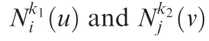
Fig.13 shows some geometric comparisons between the traditional offset surface and the interface surface obtained by our optimization method.In Fig.13,the heat map represents the Gaussian curvature of the surfaces.For the traditional offset surface,as shown in Fig.13(a),since the offset distance is small,its differential information is similar to that of the nominal surfaceSf.The varied curvature in such a case suggests that,for the roughing process,there could be dramatic changes in the depth of cut,which in turn may result in unsteady feed rate and eventually reduce the machining efficiency in roughing.On the contrary,the optimized interface surface displayed in Fig.13(b)and(c)is smoother,and has less curvature variation and hence a more uniform distribution of depth of cut,which will help reduce the kinematical loading on the machine’s axes,making it possible to assign high feed rate.In addition to the curvature,for the three interface surfaces,Fig.14 displays the distance betweenSrandSfinz-axis of the WCS.

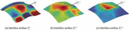
Fig.13 Interface surface Srwith heat map of Gaussian curvature of example 1.

Fig.14 Interface surface Srwith heat map representing z-distance between Srand nominal surface Sfof example 1.

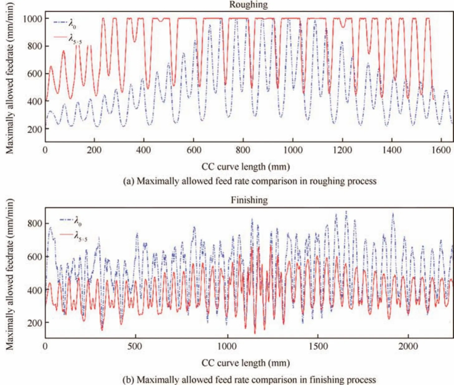
Fig.15 Comparison of maximally allowed feed rate for roughing and finishing process between traditional simple offset surface method and optimized interface surface method of example 1.

Let us now give a detailed analysis on the optimization process.Refer to Fig.15,which shows the maximally allowed feed rates’profiles along the CC curves for the three-axis roughing and five-axis finishing tool path before and after the optimization of interface surfaceSr.As the finishing tool path remains unchanged,the corresponding CC curve length remains unchanged as well during the entire optimization process.However,the interface surface can affect the total CC curve length of the roughing.As shown at the top in Fig.15,indeed the total CC curve length of the roughing process is reduced after the optimization.Moreover,even though the kinematical constraint remains unchanged during the finishing cutting,the deflection cutting force constraint varies with the change ofSrduring both the roughing and finishing process.The result of the optimization is that a more aggressive feed rate is allowed in the roughing process since the deflection cutting force is now smaller.On the contrary,the maximally allowed feed rate profile after the optimization decreases slightly(see the bottom figure in Fig.15)in the finishing process since the feed rate is now mostly dominated by the cutting force constraint which is now more stringent.Therefore,on one hand,the total CC curve length is reduced in the roughing process;on the other hand,the decrease of the feed rate in the finishing process is compensated by its increase in the roughing.Overall,the optimized interface surface achieves a 20%reduction in total machining time from the initial one.(The user-de fined maximum feed rate is set at λp=1000 mm/min for the roughing process.)

Fig.16 displays the three-axis roughing tool path for the final interface surfaceSr(Fig.16(a))and the CC curves together with some tool postures of the five-axis finishing tool path for the nominal surfaceSf(Fig.16(b)).It is worth noting that,while the finishing tool path remains fixed and irrelevant toSr,the change ofSrdoes affect the feed rate assigned to it.On the other hand,for the roughing process,the change ofSrwill affect both the tool path and the feed rate.

With the generated tool paths for the optimized interface surfaceSrand the nominal surfaceSf,the corresponding G-code part programs are then physically executed on the JDGR200_A10H five-axis machine tool(as shown in Fig.8).

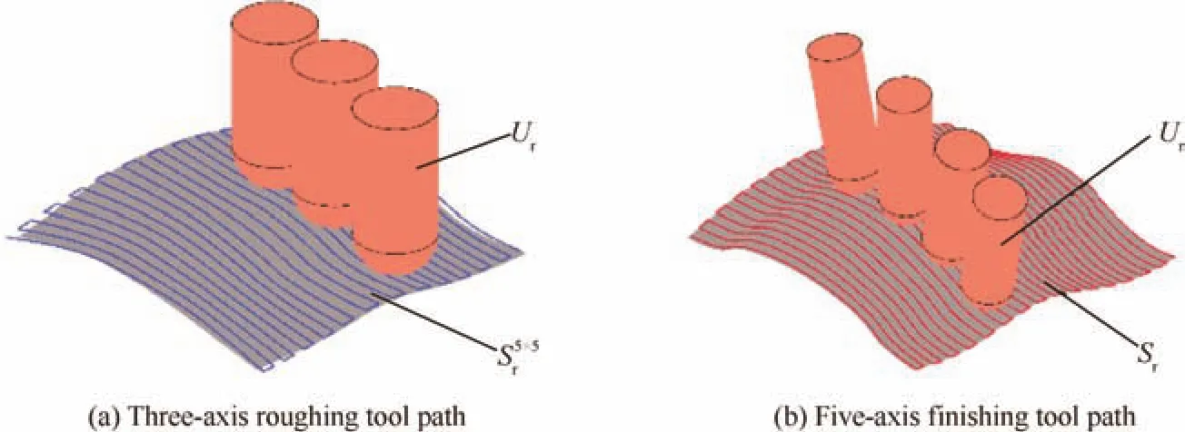
Fig.16 Generated tool paths of example 1.

Table 1 Machining time comparison of example 1.

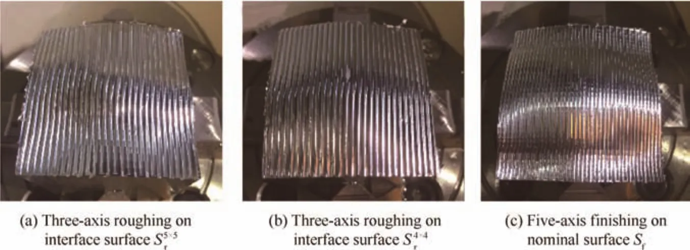
Fig.17 Photos of machined parts of example 1.

Fig.18 Freeform surface of example 2.

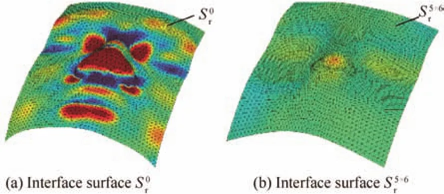
Fig.19 Interface surface Srwith heap map of Gaussian curvature of example 2.

Fig.20 Interface surface Srwith heat map representing zdistance between Srand nominal surface Sfof example 2.

The second test surfaceSfis a complex human face with dramatic curvature variation,as shown in Fig.18.The machining parameters for conducting the experiment on this surface are as follows:two ball-end cutters(UrandUf)with radiusRr=3 mm andRf=1 mm are chosen as the cutters for the roughing and finishing process,respectively;the scallop-heighthrfor roughing andhffor finishing are 0.1 mm and 0.05 mm respectively;the maximum allowed deflection cutting forces are 500 N(forUr)and 200 N(forUf).The interface surface is modeled as a B-spline surface with 5×6 control points.The rest of the experimental setting is the same as that for the first test surface.The heat maps of surface curvature and thez-distance betweenSrandSfare shown in Figs.19 and 20 respectively.Again,the raw surfaceS0is a flat face parallel to thexy-plane and 0.5 mm above the highest point onSf.

Once the optimized interface surfaceSris found,the isoplanar tool paths for rough cuttingSrand finish cuttingSfare also generated,as shown in Fig.21(a)and(b)respectively,together with the finally assigned feed rate for the tool paths.Physical cuttings are then carried out.Fig.22 shows some photos of the machined interface surfaceSrand the machined nominal surfaceSf,whereas the test data are given in Table 2.This time,in terms of real recorded total machining time,a remarkable 21%saving is achieved by the optimizedSras compared to the traditional offset surface.

Fig.22 Photos of machined parts of example 2.

Fig.21 Generated tool paths of example 2.

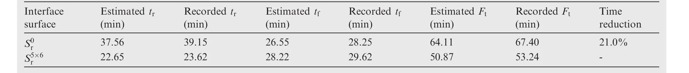
Table 2 Machining time comparison of example 2.

Finally,we would like to note that,although in the current work both roughing and finishing tool paths are required to be of iso-planar type,our interface surface optimization method actually is not limited by the tool path generation strategies.There are obviously other possible strategies for roughing and finishing and selecting a proper cutting strategy(such as the follow periphery,the follow part or zig-zag strategy)has direct impact on the eventual machining time and finish surface quality.Therefore,given a different combination of cutting strategies for roughing and finishing(e.g.,using the follow-periphery contouring milling for roughing and the iso-planar milling for finishing),as long as the tool path is generated,the IPW updating strategy is still valid in finding the maximally allowed feed rate.By solving the optimization problem of Eq.(30),the optimized interface surface can be found to minimize the total machining time of both roughing and finishing.

7.Conclusions

In this paper,we have studied the fundamental problem of how to plan the roughing and finishing process for multi-axis machining of an arbitrary freeform surface so that the total machining time can be minimized,subject to the kinematical constraints of the specific machine tool and the deflection cutting force threshold on the cutter.With respect to the specific tool path type of iso-planar milling for both roughing and finishing,we have shown that such a minimization problem is equivalent to finding a best interface surface between the roughing and finishing,and subsequently presented an optimization algorithm for finding this best interface surface.The algorithm crucially relies on an elaborate and efficient calculation of the in-process workpiece as well as the correct modeling and calculation of the cutting force in five-axis machining,and the test data from the physical cutting experiments performed by us convincingly validate the soundness of our mathematical model as well as the optimization algorithm itself.Both computer simulations and physical cutting experiments of the proposed optimization method show that substantial(+20%in our tests)savings in total machining time could be achieved as compared to the traditional simple offset surface method.

Regarding the future work,several issues remain to be addressed.First,the iso-planar tool path is adopted as the pre-determined type of machining for both roughing and finishing process.Understandably however,under the same machining parameters such as the tool sizes and scallopheight,some other types of tool path such as the iso-scallop height or contouring might lead to better results than our current one.Secondly,as the roughing process is of three-axis type,the interface surface is indeed a monotone one,but it does not have to be monotone with respect to thexy-plane of WCS,as is assumed in the current algorithm.Finally,in this work the entire roughing process is made of a single round of milling,although in practice several rounds of milling are usually applied,each of which requires its own interface surface.

Appendix A.Supplementary material

Supplementary data associated with this article can be found,in the online version,at http://dx.doi.org/10.1016/j.cja.2017.07.004.

1.Elber G,Cohen E.Toolpath generation for freeform surface models.Comput Des1994;26(6):490–6.

2.Sun YW,Jia ZY,Ren F,Guo DM.Adaptive feedrate scheduling for NC machining along curvilinear paths with improved kinematic and geometric properties.Int J Adv Manuf Technol2006;36(1–2):60–8.

3.Zhao JB,Zou Q,Li L,Zhou B.Tool path planning based on conformal parameterization for meshes.Chin J Aeronaut2015;28(5):1555–63.

4.Cho JH,Kim JW,Kim K.CNC tool path planning for multipatch sculptured surfaces.Int J Prod Res2000;38(7):1677–87.

5.Ding S,Mannan MA,Poo AN,Yang DCH,Han Z.Adaptive isoplanar tool path generation for machining of free-form surfaces.Comput Des2003;35(2):141–53.

6.Feng HY,Teng ZJ.Iso-planar piecewise linear NC tool path generation from discrete measured data points.Comput Des2005;37(1):55–64.

7.Chen T,Shi ZL.A tool path generation strategy for three-axis ball-end milling of free-form surfaces.J Mater Process Technol2008;208(1–3):259–63.

8.Suresh K,Yang DCH.Constant scallop-height machining of freeform surfaces.J Eng Ind1994;116(2):253–9.

9.Lee E.Contour offset approach to spiral toolpath generation with constant scallop height.Comput Des2003;35(6):511–8.

10.Li H,Feng HY.Efficient five-axis machining of free-form surfaces with constant scallop height tool paths.Int J Prod Res2004;42(12):2403–17.

11.Lin RS,Koren Y.Efficient tool-path planning for machining freeform surfaces.J Eng Ind1996;118(1):20–8.

12.Giri V,Bezbaruah D,Bubna P,Roy Choudhury A.Selection of master cutter paths in sculptured surface machining by employing curvature principle.Int J Mach Tools Manuf2005;45(10):1202–9.

13.Agrawal RK,Pratihar DK,Roy CA.Optimization of CNC isoscallop free form surface machining using a genetic algorithm.Int J Mach Tools Manuf2006;46(7–8):811–9.

14.Lin ZW,Fu JZ,Shen HY,Gan WF.A generic uniform scallop tool path generation method for five-axis machining of freeform surface.Comput Des2014;56:120–32.

15.Kim T,Sarma SE.Toolpath generation along directions of maximum kinematic performance;a first cut at machine-optimal paths.Comput Des2002;34(6):453–68.

16.Sencer B,Altintas Y,Croft E.Feed optimization for five-axis CNC machine tools with drive constraints.Int J Mach Tools Manuf2008;48(7–8):733–45.

17.Beudaert X,Pechard PY,Tournier C.5-Axis tool path smoothing based on drive constraints.Int J Mach Tools Manuf2011;51(12):958–65.

18.Sun YW,Zhao Y,Bao YR,Guo DM.A novel adaptive-feedrate interpolation method for NURBS tool path with drive constraints.Int J Mach Tools Manuf2014;77:74–81.

19.Hu PC,Tang K.Five-axis tool path generation based on machinedependent potential field.Int J Comput Integr Manuf2016;29(6):636–51.

20.Lee P,Altintas Y.Prediction of ball-end milling forces from orthogonal cutting data.Int J Mach Tools Manuf1996;36(9):1059–72.

21.Li YW,Liang SY.Cutting force analysis in transient state milling processes.Int J Adv Manuf Technol1999;15(11):785–90.

22.Engin S,Altintas Y.Mechanics and dynamics of general milling cutters.:Part I:helical end mills.Int J Mach Tools Manuf2001;41(15):2195–212.

23.Boz Y,Erdim H,Lazoglu I.Modeling cutting forces for 5-axis machining of sculptured surfaces.Adv Mater Res2011;223:701–12.

24.Lamikiz A,Lo´pez de Lacalle LN,Sa´nchez JA,Salgado MA.Cutting force estimation in sculptured surface milling.Int J Mach Tools Manuf2004;44(14):1511–26.

25.Kim GM,Cho PJ,Chu CN.Cutting force prediction of sculptured surface ball-end milling using Z-map.Int J Mach Tools Manuf2000;40(2):277–91.

26.Zhu RX,Kapoor SG,DeVor RE.Mechanistic modeling of the ball end milling process for multi-axis machining of free-form surfaces.J Manuf Sci Eng2001;123(3):369–79.

27.Fussell BK,Jerard RB,Hemmett JG.Modeling of cutting geometry and forces for 5-axis sculptured surface machining.Comput Des2003;35(4):333–46.

28.Sun YW,Guo Q.Numerical simulation and prediction of cutting forces in five-axis milling processes with cutter run-out.Int J Mach Tools Manuf2011;51(10–11):806–15.

29.Li ZL,Niu JB,Wang XZ,Zhu LM.Mechanistic modeling of fiveaxis machining with a general end mill considering cutter runout.Int J Mach Tools Manuf2015;96:67–79.

30.Kurt M,Bagci E.Feedrate optimisation/scheduling on sculptured surface machining:a comprehensive review,applications and future directions.Int J Adv Manuf Technol2011;55(9):1037–67.

31.Zeroudi N,Fontaine M.Prediction of tool deflection and tool path compensation in ball-end milling.J Intell Manuf2015;26(3):425–45.

32.Kim GM,Kim BH,Chu CN.Estimation of cutter deflection and form error in ball-end milling processes.Int J Mach Tools Manuf2003;43(9):917–24.

33.Xu K,Tang K.Five-axis tool path and feed rate optimization based on the cutting force-area quotient potential field.Int J Adv Manuf Technol2014;75(9):1661–79.

34.Tao SB,Ting KL.Uni fied rough cutting tool path generation for sculptured surface machining.Int J Prod Res2001;39(13):2973–89.

35.Lefebvre PP,Lauwers B.3D Morphing for generating intermediate roughing levels in multi-axis machining.Comput Aided Des Appl2005;2(1–4):115–23.

36.Xu K,Tang K.An energy saving approach for rough milling tool path planning.Comput Aided Des Appl2016;13(2):253–64.

37.Tang M,Zhang DH,Luo M,Wu BH.Tool path generation for clean-up machining of impeller by point-searching based method.Chin J Aeronaut2012;25(1):131–6.

38.Hu PC,Tang K.Improving the dynamics of five-axis machining through optimization of workpiece setup and tool orientations.Comput Des2011;43(12):1693–706.

39.Jerard RB,Drysdale RL,Hauck KE,Schaudt B,Magewick J.Methods for detecting errors in numerically controlled machining of sculptured surfaces.IEEE Comput Graph Appl1989;9(1):26–39.