Three-dimensional Fusion of Spaceborne and Ground Radar Reflectivity Data Using a Neural Network–Based Approach

Leilei KOU,Zhuihui WANG,and Fen XU

1Key Laboratory of Meteorological Disaster,Ministry of Education/Joint International Research Laboratory of Climate and Environment Change/Collaborative Innovation Center on Forecast and Evaluation of Meteorological Disasters,Nanjing University of Information Science and Technology,Nanjing 210044,China

2Meteorological Bureau of Jiangsu Province,Nanjing 210008,China

1.Introduction

The horizontal and vertical structure of radar echoes are importantindicatorsoftheorganizationofprecipitatingcloud systems.The horizontal structure to a certain degree re-flects the properties and status of precipitating clouds,and the vertical structure is an indicator of the thermodynamic processes,dynamic processes,and microphysics of precipitation(Steiner et al.,1995;Fu et al.,2003).It is essential to obtain and analyze the 3D structure of radar echoes at high spatial resolution,especially for the recognition,tracking and forecasting of convective storms.Precipitation structure can be captured through radars on different platforms,such as on the ground or onboard satellites.A major purpose of the deployment of ground-based weather radars is to locate storms and detect their inner structures,and then quantitatively estimate the precipitation generated.The precipitation radar(PR)onboard the Tropical Rainfall Measuring Mission(TRMM)satellite was thefirst spaceborne weather radar,and the availability of spaceborne precipitation radar is a great asset for the observation of precipitation.However,each remote source of observations has some advantages and limitations.TRMM PR can provide reflectivity data at a fine vertical resolution of 250 m;plus,TRMM PR data are welldistributed and are unrestricted by beam blockage and the cone of silence(Kozu et al.,2001;Liao et al.,2001).However,it has a low sensitivity threshold of 18 dBZ.Compared with TRMM PR,ground radar(GR)has relatively good capability in detecting weak precipitation and a relatively good horizontal resolution,but GR measurements are approximately horizontal in their scanning,meaning a low variable vertical resolution and blind zones are typical(Zhang et al.,2005;Gupta et al.,2006).To obtain a 3D high-resolution precipitation structure,a possible solution is to merge GR andTRMMPRmeasurementsandexploittheadvantagesthat each measurement technique has to offer.

There are numerous research scientists who are working on algorithms and techniques for combining data from spaceborne and ground-based precipitation radar(Calheiros et al.,2000;Gupta et al.,2006;Mahani and Khanbilvardi,2009;Gourley et al.,2010;Dolan et al.,2011;Ebtehaj and Foufoula-Georgiou,2011;Chandrasekar and Cifelli,2012;Wen et al.,2013;Cao et al.,2014;Kou et al.,2014,2016;Lee et al.,2015;Verdin et al.,2015;Wang et al.,2015).In Ebtehaj and Foufoula-Georgiou(2011),multiscale multisensory precipitation data fusion were developed using precipitation reflectivity images from TRMM PR and GR in wavelet domains.In Kou et al.(2014),TRMM PR reflectivity data and Nanjing GR data were blended with a simple averaging algorithm and a maximum fusion method to obtain a more complete echo structure.Cao et al.(2014)and Wen et al.(2013)proposed a vertical profile of reflectivity identification and enhancement approach to improve GR quantitative precipitation estimation(QPE),which integrates NOAA’s National Mosaic QPE system and NASA’s TRMM PR measurements.Verdin et al.(2015)used a Bayesian kriging approach to blend satellite and ground precipitation observations to improve rainfall estimation.Most efforts in using information from multiple sensors have been aimed at producing more accurate QPE by calibrating or merging GR-based and satellitebased rainfall with rain gauge observations(Xiao and Chandrasekar,1997;Xu and Chandrasekar,2005;Li et al.,2013;Cao et al.,2014;Chandrasekar et al.,2014;Nielsen et al.,2014;Pan et al.,2015).In the present study,we merge reflectivity data from GR and TRMM PR to obtain the 3D radar echo structure at high spatial resolution.3D high-resolution reflectivity data are important for detecting and analyzing convective storms,and can also serve as an important source in data assimilation for convective-scale numerical weather modeling.Generally,3D radar echo images are obtained from gridding GR volume scanning data with interpolation algorithms.The commonly used interpolation techniques include:nearest neighbor,linear interpolation,and the Barnes or exponential weighting scheme(Zhang et al.,2005).However,GR data are limited by their volume coverage pattern and beam broadening with increasing range;therefore,the vertical resolution of the 3D reflectivity field is still very low after interpolation.

The goal of the present study is to generate a more complete3Dradarreflectivityfield withfinerspatialresolutionby merging spaceborne and ground-based radar measurements using a neural network(NN)–based approach.NN algorithms have been widely applied in rainfall forecasting and estimation,using radar reflectivity data at different times as inputs and targets,respectively,or using radar data as inputs and rain gauge data as the target(Hall et al.,1999;Orlandini and Morlini,2000;Liu et al.,2001;Sarma et al.,2008;de Oliveira et al.,2009;Chen et al.,2010;Alqudah et al.,2013).Inthepresentstudy,3DgriddedGRreflectivitydataafterhorizontal downsampling serve as the input for NN training,and 3D high vertical resolution TRMM PR reflectivity data are the target.Thus,the relationship between GR and TRMM PR reflectivity data is established.The trained NNs are then used to obtain 3D high resolution reflectivity from the original GR gridded data with high horizontal resolution.Owing to the low sensitivity(18 dBZ)of TRMM PR,we only use data greater than 18 dBZ during the NN training and application process.Those data below PR’s sensitivity are obtained from the vertical interpolation of corresponding GR data.Besides,the blind areas(cone of silence)of the GR data,caused by the GR volume scan mode,are also considered in the 3D fusion of TRMM PR and GR.The reflectivity data over the GR blind areas are compensated by blending the TRMM PR data in the blind areas and their neighboring GR data with a distance weighting–based approach.After combining the fused reflectivity data obtained with the NN method,the interpolated data below PR’s sensitivity and the compensated reflectivity data over the cone of silence of GR,a complete 3Dhigh-resolution radar reflectivitydataset is generated.The proposed algorithm is evaluated based on a convective precipitation event,and the generated high-resolution 3D fused reflectivity data are compared with the horizontal and vertical cross sections of TRMM PR and GR with an interpolation algorithm to preliminarily assess their performance and characteristics.

2.Data preprocessing

2.1.Data selection and quality control

TheselectedareaiscenteredattheNanjingradarsitewith a 150-km radius.Since the time of one volume scan of the GR is about 6 min,the GR volume scan is acquired beginning within a 6-min window centered on the TRMM PR overpass time,along with its corresponding spaceborne radar data.

The level II algorithm of the PR profile(2A25),which includes ground clutterfiltering,attenuation and beam filling correction,is applied to the TRMM PR reflectivity data.This relies on the output of 1C21 and 1B21 to separate the surface clutter ranges from the clutter-free ranges(Kozu et al.,2001;Wang et al.,2015).The clutter identification routine used in 1B21 may not be perfect,and some surface clutter may occasionally be misidentified as rain echo in 2A25,but this problem is usually confined to mountain regions.Moreover,only the data at a height above 1 km are used,which may further minimize the contamination from the remaining ground clutter.The TRMM PR attenuation correction is processed with a Hitschfeld–Bordan iterative scheme and surface reference technique(Iguchi et al.,2000;Meneghini et al.,2004),and the beamfilling correction is also performed in the 2A25 product(Iguchi et al.,2000;Kozu et al.,2001).TRMM PR operates at 13.8 GHz(Ku band)and has a low sensitivity threshold of 18 dBZ.It scans 17◦to either side of nadir at intervals of 0.7◦in the cross-track direction,which gives a swath width of 214 km(246 km after boost)at the Earth’s surface,with a horizontal resolution of about 4.3 km(5 km after boost)at nadir.The TRMM PR pulse duration is 1.67µs,which gives a vertical resolution of about 0.25 km.

For this case study,the GR data from ground Doppler radar at Longwang Mountain(32.1908◦N,118.6969◦E)in Nanjing city,China,are adopted.Nanjing radar operates at the S band with a VCP21 mode.The current reflectivity product operates at a 1-km range resolution and 1◦azimuthal resolution,with a minimum detectable reflectivity of−7.5 dBZ at 50 km.Before fusing the GR data,quality control is performed on the Nanjing GR reflectivity data,including removing electronic interference,anomalous propagations and ground clutter,and system bias correction.The NCAR SOLO II algorithm is used to remove the anomalous propagations and ground clutter,and the system bias correction is addressed in section 2.3.

2.2.Gridding and matching

For the subsequent data fusion,the TRMM PR and GR reflectivity data should be interpolated in a common coordinate system.The spatial matchup scheme is based on the grid matching method provided in the literature related to comparisons of PR and GR(Anagnostou et al.,2001;Liao and Meneghini,2009;Wang and Wolff,2009).The gridded GR data in a 3D Cartesian coordinate system are interpolated from the GR spherical coordinate system centered at the GR using a cubic linear interpolation algorithm,with a vertical resolution of about 1 km to a height of 20 km and a horizontal resolution of about 1 km to a horizontal extent of±150 km.Thus,3D gridded data for Nanjing GR are obtained with a resolution of about 1 km×1 km×1 km.

The TRMM PR data are also resampled into Cartesian coordinates.During 3D gridding,the displacement or parallax of PR samples is corrected with the method described in Wang and Wolff(2009).After displacement correction,the resolution of resampled TRMM PR in a 3D grid is about 4 km×4 km×0.25 km.

A case study for Nanjing GR on 27 May 2008 is performed,and the orbit number is 59995.The overpass time of PR at Nanjing GR is 0456:41 UTC,and the beginning time of the corresponding GR volume scan is 0453:00 UTC.Figure 1a shows the GR CAPPI(Constant Altitude Plan Position Indicator)data at 3 km height with a resolution of 1 km×1 km.Figure 1b shows the PR data at 3 km height in Cartesian coordinates with a resolution of 4 km×4 km.For the following NN training,the input GR data should be downsampled to the same resolution as the PR horizontal resolution.The downsampled GR reflectivity is shown in Figure.1c with a horizontal resolution 4 km×4 km using an averagefilter of size 4×4 on a horizontal plane.

It can be seen that the radar echoes from TRMM PR are basically consistent with those from GR in Fig.1.Figure 2 is a scatter plot of TRMM PR and gridded GR reflectivity at 3 km height in Figs.1b and c.The correlation coefficient of downsampled GR data and original TRMM PR data is 0.79,indicating relatively high coherence,but the mean difference(PR minus GR)is about 2.9 dB.Many factors,like differences in radar sensitivities,sample volumes,viewing angles,attenuation and different radar wavelengths,may influence the reflectivity difference of TRMM PR and GR,but the GR system calibration bias may bring about the difference between TRMM PR and GR(Anagnostou et al.,2001).

2.3.GR calibration bias correction

For NN fusion processing,the GR reflectivity data and TRMM PR data are assumed as unbiased estimates in a global sense,and hence the system calibration bias should be corrected if it exists.With considerable long-term certainty and stability,the TRMM PR has served as a reference to calibrate GRs and to detect inconsistencies between adjacent GRs(Anagnostou et al.,2001;Bolen and Chandrasekar,2000;Wang and Wolff,2009).In Zhu et al.(2016),245 TRMM PR and Nanjing GR matchup cases for the period 2008–13 were adopted and compared using statistical analysis methods to determine the calibration biases of Nanjing GR.The results showed that Nanjing GR presents a“threestage”feature,and the mean deviation of TRMM PR and Nanjing GR in stage 1 from January 2008 to March 2010 was about 1.2 dB,the mean deviation in stage 2 from March 2010 to May 2013 was about 4.2 dB,and the mean deviation in stage 3 from May 2013 to October 2013 was approximately 1.5 dB.In this study,a bias adjustment of 1.2 dB is applied to GR for the case in Figure.1.

2.4.Conversion from Ku to S band

Fig.1.(a)Gridded Nanjing GR with horizontal resolution of 1 km×1 km;(b)TRMM PR with horizontal resolution of 4 km×4 km;and(c)gridded Nanjing GR downsampled by a factor of 4 at a height of 3 km.

Fig.2.Scatterplot of TRMM PR and GR reflectivity.The data are the common data from 3 km CAPPI in Figs.1b and c.The straight line is the regression line,and the sample points,the correlation coefficients,and the mean error between TRMM PR and GR reflectivity are shown in the inset text.

For TRMM PR at Ku band,some large particles may fall into the Mie scattering region,and the radar reflectivity factors at S and Ku bands can be significantly different(Liao and Meneghini,2009;Wen et al.,2011;Cao et al.,2013).This Mie scattering effect can be estimated using a raindrop size distribution model.Based on the gamma particle size distribution modeling in the ice region,melting layer,and raining region,Cao et al.(2013)derived the empirical relations between Ku and S band reflectivity in different regions.Since the proposed algorithm is mainly for convective precipitation,here we divide the precipitation into snow and rain regions according to the height of the freezing level in the 2A23 product of TRMM PR,and the melting region is not calculated separately:

where Zsand ZKuare expressed in dBZ units.From the relations in Eq.(1),a Ku band reflectivity can be conveniently converted to an S band reflectivity.Based on Eq.(1),it can be seen that the difference between Zsand ZKuis small when Zs<35 dBZ,and about 2 dB or more when Zs>35 dBZ.

3. 3D fusion of TRMM PR and GR reflectivity data

The NN is trained using downsampled 3D gridded GR data(4 km×4 km×1 km)as the input,and high vertical resolution PR data(4 km×4 km×0.25 km)as the target.The trained NN is then applied to the original gridded GR data with a resolution of 1 km×1 km×1 km,and 1 km×1 km× 0.25 km fused reflectivity data can be obtained.During the fusionwiththeNNapproach,weonlyusethereflectivitydata greater than PR’s sensitivity(18 dBZ).Besides the data with NN fusion,there are reflectivity data less than 18 dBZ,GR data outside the TRMM PR scanning area,and missing data within GR blind areas that are caused by the limited elevation angles of GR volume scanning.For the data less than 18 dBZ and the data outside the TRMM PR swath,they are obtained with linear interpolation of corresponding preprocessed GR data.The data within GR blind areas are produced by merging TRMM PR data at coinciding locations and neighboring GR data after NN fusion.Then,a complete 3D high resolution reflectivity dataset can be generated.A generalflow chart of the 3D fusion of TRMM PR and GR reflectivity data is shown in Figure.3.Thefirst four steps in Figure.3 have been described in section 2.The next four steps are discussed in the following sections.

3.1.Fusion with NN

NNs have been exploited in weather radar applications like precipitation forecasting,rainfall rate estimation,wind prediction,and so on(Orlandini and Morlini,2000;Sarma et al.,2008;Wang et al.,2015).A new NN approach is developed where multiple NNs are trained using the 0.25 km vertical resolution TRMM PR data at different heights as outputs of training NNs,and gridded GR data with 1 km vertical resolution at different heights as inputs.Different from conventional NN methods,the goal of this study is to gain a 3D high resolution radar echo structure,and hence the 3D gridded radar reflectivity data with different resolution are used as inputs and outputs for training NNs,respectively.

Fig.3.Overall schematicflow diagram of 3D fusion of TRMM PR and GR reflectivity data.

Fig.4.Flow chart of the Kth NN fusion,where K=2–18.The upper part is the NN training part,and the lower dashed box part applies the trained NN parameters to retrieve high vertical resolution reflectivity data with inputs of original GR data.A total of 19 NNs are modeled for training 20 layers of GR data with a vertical resolution of 1 km and 77 layers of TRMM PR data with a vertical resolution of 1 km.The inputs of thefirst and 19th NN are GR data at heights of 1 km,2 km,3 km and 4 km,and heights of 17 km,18 km,19 km and 20 km,respectively.

The vertical range of the 3D reflectivity data is from 1 km to 20 km,and thus the number of layers is 20 for the GR data with a vertical resolution of 1 km,and the number of layers is 77 for the TRMM PR data with a vertical resolution of 0.25 km.For one NN,we use TRMM PR data at four adjacent heights as outputs,and GR data at 4 heights nearest to the output heights as inputs.In this way,19 neural networks are trained with 20 layers of GR data and 77 layers of TRMM PR data.The specific structure setting for the Kth neural network is shown in Fig.4.In Fig.4,the input of the Kth training NN is 2D GR data at four heights of K−1 km,K km,K+1 km and K+2 km,and the corresponding output is TRMM PR data at four heights of K km,K+0.25 km,K+0.5 km and K+0.75 km,where K=2–18.Here,thefirst and the 19th NN are excluded.The inputs of thefirst NN are GR data at heights of 1 km,2 km,3 km and 4 km,and the corresponding outputs are TRMM PR data at heights of 1 km,1.25 km,1.5 km and 1.75 km.For the 19th neural network,the inputs are GR data at heights of 17 km,18 km,19 km and 20 km,and the outputs are TRMM PR data at heights of 19 km,19.25 km,19.5 km,19.75 km and 20 km.Besides,for matching to the horizontal resolution of TRMM PR data,original GR data are converted to 4 km×4 km by smoothing and downsampling by a factor of 4,using an averagefilter of size 4×4.After 19 NNs are trained,the trained NN parameters are applied to the original 2D GR data,and the output data with a high vertical resolution of 0.25 km and horizontal resolution of 1 km×1 km can be generated.

The upper part of Fig.4 is the NN training part,and the application part uses the trained NN parameters to retrieve high vertical resolution reflectivity data with an input of high horizontal resolution GR data.The inner structure of the Kth training NN is shown in Fig.5.

ThetypesofNNusedinFig.5areback-propagationfeedforward NNs.In the following,the fundamental algorithm of the back-propagation NN is simply reviewed.After normalization of input data,the data in the hidden layer are updated with weighting,and the outputs of the hidden layerare calculated with a logistic sigmoid activation function,

For weighting matrices and adjusting factors in the hidden and output layer,they are updated according to Levenberg–

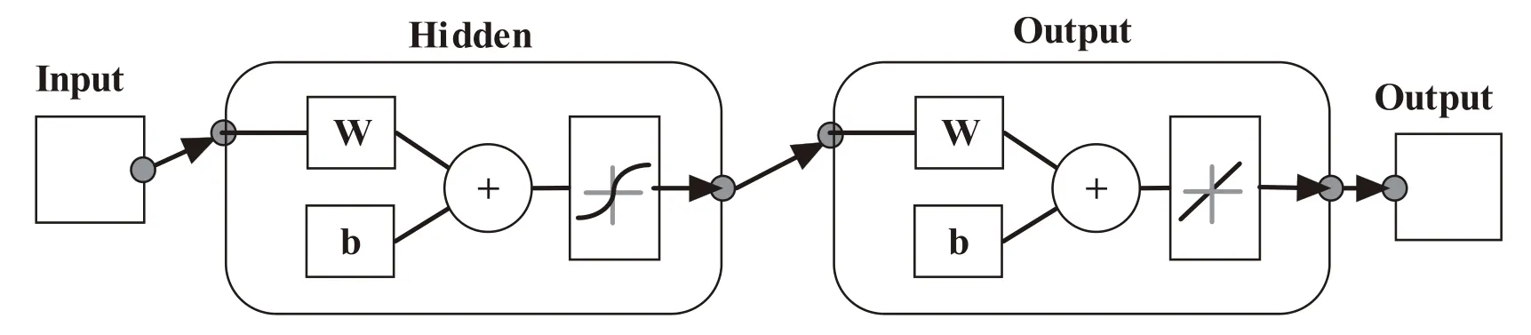
Fig.5.Inner structure of the training NN.Three layers are included in the training NN,which are the input layer,hidden layer and output layer.The W and b in the hidden layer and output layer are the weighting matrix and adjusting factor,respectively.The outputs of the hidden layer are calculated with a logistic sigmoid activation function,and the outputs of the output layer are calculated with a linear activation function.

Marquardt optimization,

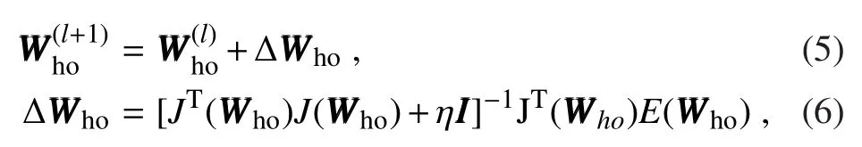
where l represents the lth iteration,T indicates transposition,η is the learning rate, I is the identity matrix,andis the Jacobian matrix ofis the vector of the

where n is number of nodes of the output layer.From Fig.4,it is seen that n is 4.Also,we can see that the size of the input matrixis 4×M and the size of the output matrixis 4×M,where M is the data samples(matched GR and PR data)in one training set.It should be noted that only commonly available data in the matched area of the four input height layers of the GR data and output TRMM PR data are used during NN training.The weighting matrices of the hidden layerand adjusting factors(b b b)are updated similarly to that ofFinally,the global error of the network is calculated with

If the error e reaches setting precision or learning times larger than the setting maximum number of iterations or error e no longer converges,the algorithm stops.If not,the next iteration starts until one of the aforementioned conditions has been satisfied.The trained results of the weighting matrices and adjusting factors are saved for the application of the trained NN.

Figure 6a is a plot of MSE(mean square error)variation of the training process for the third NN.The input data are 2D gridded GR at heights of 2 km,3 km,4 km and 5 km,and the corresponding output is 2D TRMM PR data at heights of 3 km,3.25 km,3.5 km and 3.75 km.The MSE converges to 0.025284 dB2at the 21st iteration.For this NN training,the number of hidden layer nodes is set as nine.

The performance or the generalization ability of NN training is dependent on many factors,such as the issue complexity,the data samples and the number of hidden layer nodes.Thefirst two factors are difficult to change for a given case,and the optimum number of hidden layer nodes is also usually difficult to determine.Generally,some empirical formulas for obtaining hidden layer nodes are used,like(Shi et al.,2009)

where m is number of input nodes,n is the number of output nodes,L is the number of hidden layer nodes,and α is a number between 1 and 10.Equation(9)is just empirical formulas,which has certain limitations because it ignores the size of training samples and complexity of the issue.In practical applications,we can use the trial and error method by testing the range of the formulas in Eq.(9)to obtain a relatively optimal number for each NN.For four input nodes and four output nodes in Fig.5,the number of hidden layer nodes we can try is 4–12.Besides,the optimum number of hidden layer nodes may be determined by optimization algorithms like a genetic algorithm or a particle swarm optimization algorithm.Since different types of precipitation may vary distinctly,the matched available training pairs are separated into stratiform and convective types according to the parameter“rainType”in the TRMM PR 2A23 product,and the rain type classification is shown in Fig.6b.Figure 6c is the global MSE of 19 trained NNs with relatively optimal hidden layer nodes determined by the trial and error method,and Fig.6d is the number of samples of convective and stratiform rain for 19 NNs.From Fig.6c it is apparent that the performance of training NN reduces with the increase in height,and the performance of convective rain is superior to that of stratiform rain at higher heights.Since the case in this study is a thunderstorm event primarily featuring convective rain,the number of stratiform precipitation samples that can be seen from Fig.6d decreases sharply(the number falls back into single digits)at higher heights,which makes the performance of stratiform rain become very poor at heights above 9 km.

Fig.6.(a)Performance variation of the training process for the third NN.The MSE converges to 0.025284 dB2at the 21st iteration.(b)Rain type classification,where plus signs represent convective precipitation and dots stratiform precipitation.(c)Convergent global MSE(dB2)of 19 trained NNs.(d)Number of samples for convective and stratiform precipitation of 19 training NNs.Since different types of precipitation may vary distinctly,the matched available training pairs are separated into stratiform(black line)and convective types(red line).The precipitation types are determined according to the rain type classification in the TRMM PR 2A23 products.

Of note is that the small training dataset potentially limits the usefulness of the NN approach.In the NN training,the critical minimal data samples are generally required to be at least twice the number of NN weights(Shi et al.,2009).In the case of Fig.6b,the numbers of convective and stratiform data samples for the 10th NN are 59 and 10 respectively,and so the samples are not enough for training even if precipitation data are not separated into different types.Hence,the NNs greater than the 10th(10–19 NNs)are regarded as un-fit for NN training.The high-resolution reflectivity of 10–19 NNs is obtained with interpolation and simple linear fusion.Firstly,GR data above 10 km height are processed with linear interpolation in the vertical direction to produce a 0.25 km height resolution.Then,TRMM PR data above 10 km height are processed with nearest neighbor interpolation in the horizontal direction to produce a 1 km×1 km horizontal resolution.Finally,the high-resolution fusion data at the Nth(N>10 for this case)height are obtained with

where fGRNand fPRNare the reflectivity of GR and TRMM PR at the Nth height,respectively;N is from 10 to 20 with aspacing of 0.25;andandrepresent averaging over the common echoes of the Nth height GR and TRMM PR data,respectively.

3.2.Weak echoes interpolation

The minimum detectable reflectivity of TRMM PR is about 18 dBZ,and data less than this minimum are excluded from the NN training,so weak echoes less than 18 dBZ cannot be obtained with the NN method.The echoes less than 18 dBZ may be used to estimate the height of the storm top and,most importantly,they are utilized to estimate the rainfall amount.So,the weak echoes should be taken into account for the 3D fusion of TRMM PR and GR data.Thefield below 18 dBZ in thefinal 3D high-resolution fusion reflectivity data is generated with linear interpolation in the vertical direction of the corresponding GR data.

3.3.GR blind areas compensation

Nanjing GR scans in the VCP 21 mode,and the highest elevation angle is 19.5◦.Limited by the scanning elevation angles,significant data voids exist above the highest beam,i.e.,the GR blind area or the “cone of silence”.The area of the “cone of silence”increases with height.When the storm is at 20 km horizontal distance from the radar,the radar can only detect the precipitation below the height of about 7.1 km,and the characteristic echo parameters of most convective precipitation will be underestimated.

After GR data are processed with NN fusion,the remaining GR blind area echoes are obtained by merging upsampled TRMM PR data and coincident surrounding pixels of high-resolution NN fused data in a selected window.For a given pixel in a blind area,the optimum weight can be determined by the available data and the distance between the centerpixelandneighboringpixelsfromthemergingwindow(Mahani and Khanbilvardi,2009).The window size is varied according to the size of the GR blind area and the number of surrounding reflectivity pixels.

The merging method is to adjust the TRMM PR reflectivity data for any given pixel in the blind area based on an appropriate weight with respect to the available TRMM PR and NN-fused reflectivity of its neighboring pixels.The weight factor wiis calculated by

where riis the distance between the center pixel(o)and the observation pixel(i);rois the maximum distance from the center;and(x,y)are the grid pixel coordinates.The merged reflectivity for the center pixel(fPRGRo)is obtained by

where fPRGRiand fPRiare the reflectivity of the NN-fused data(PRGRNN)and TRMM PR for the observation pixel(i)inside the window,respectively;and n is the number of pixels observed with both PRGR and TRMM PR inside the window.

The same data shown in Fig.1 are used here to illustrate the results of blind area compensation.Figure 7a shows the PRGRNNat 3 km height with a blind area of about 16×16 pixels,and Fig.7b shows the TRMM PR data upsampled by a factor of 4 with nearest neighborhood interpolation for matching with the fused data,PRGRNN.Figure 7c shows the merging result by simply substituting the blind area data with the corresponding TRMM PR data in Fig.7b.Merging Fig.7a and Fig.7b with the distance weighting–based approach,we get the merging result shown in Fig.7d with a window size of 5×5 pixels.Comparing Fig.7c with Fig.7d,it can be seen that the merging result with the distance weighting–based approach in Fig.7d is more consistent with the surrounding original data in Fig.7a than the TRMM PR data substitution in Fig.7c.That is because the merging approach retains more details on the reflectivity structures of PRGRNNby allowing more contributions from near-range observations.

3.4.Combination

3D high-resolution reflectivity data over GR regions larger than PR’s sensitivity can be obtained using NN fusion.For data below PR’s sensitivity,the high-resolution data are generated with linear interpolation in the vertical direction of the corresponding GR data.By merging upsampled TRMM PR data at each height with coincident surrounding pixels of PRGRNNdata in a selected window,high-resolution data over GR blind areas can be obtained.For convenience,the fused 3D high-resolution reflectivity data are denoted as PRGR data;the fused data without blind areas compensation is denoted as PRGRNN.

Fig.7.(a)Reflectivity data at 3 km height after NN fusion as described in section 3.1.(b)TRMM PR reflectivity data at 3 km height with a horizontal resolution of 1 km × 1 km using the nearest neighbor method.(c)Merged reflectivity images by compensating blind areas with TRMM PR data substitution.(d)Merged reflectivity images by compensating blind areas with the distance weighting–based approach with a window size of 5×5 pixels.For better revealing the compensation results,the images are enlarged around the blind areas.

Thefusedhigh-resolutionresultsareshowninFigs.8–10.Figure 8a shows the 3-km CAPPI of the original GR reflectivity data,and Fig.8c shows the fused 3D high-resolution PRGR data at 3-km height.For validating the performance of the fused result,the horizontal section of PRGR is compared with GR and TRMM PR data at each grid point with the same resolution,and original TRMM PR data are upsampled by a factor of 4 with the nearest neighborhood method shown in Fig.8b.It can be seen that the echo structure of the fused product,PRGR,is close to the GR data,and the impact of TRMM PR on the magnitude of the PRGRfield can be found in the central region of the domain in Fig.8c.Compared with upsampled TRMM PR,the fused product,PRGR,recovers more small scale features and produces a fused re-flectivity image with a more detailed structure.Besides,the weak echoes below PR’s sensitivity and the echoes within the cone of silence are included in the fusion product,which makes the echo structure more complete.A 1D reflectivity dataset shown in Fig.8d,which is obtained along the horizontal dashed line in Fig.8c,better demonstrates the performance of the PRGR data.It can be seen that the red line denoting TRMM PR data is smoother due to its coarse horizontal resolution,and the fused data preserve thefine structure of GR while taking into account information from the TRMM PR observation.

Statistical comparisons of reflectivity data in Fig.8 are shown in Table 1,where correlation coefficients(Corr.Coeff),mean errors(Mean)and root-mean-square errors(RMSEs)between TRMM PR data and GR,fused PRGR data and TRMM PR,and fused PRGR data and GR,are compared.The data pairs selected in the comparisons are in the area where both TRMM PR and GR data are available;hence,PRGR data used are mainly data with NN fusion,and Table 1 mainly quantitatively reflects the performance of the fused product with the NN fusion method.For matching to GR and PRGR data,the TRMM PR data used are the upsampled data in the horizontal direction with the nearest neighborhoodmethod.The results in Table 1 show that the generated PRGR data at horizontal planes are more correlated to GR,showing ahighcorrelationcoefficient,whichmeansthatthehorizontal structureofPRGRismoresimilartothatofGR.Themeanerror and RMSE of PRGR to TRMM PR is much smaller than that of the original GR to TRMM PR,which indicates the magnitude of PRGR with NN fusion incorporates the characteristics of TRMM PR.

Table 1.Statistical comparisons among the generated PRGR data(Fig.8c),TRMM PR(Fig.8b),and GR data(Fig.8a).

Fig.8.(a)Original GR reflectivity data;(b)upsampled TRMM PR data(horizontal resolution:1 km × 1 km)with the nearest neighbor method,and(c)fused high-resolution reflectivity data(PRGR)at 3 km height.(d)Reflectivity profiles along the dashed line in(c),where the red line denotes the TRMM PR data,the black line GR data,and the green line PRGR data.

The images in Figs.9a–d and Figs.10a–d are vertical cross sections of the reflectivity along the black solid line and dashed line in Fig.8a,where Fig.9 represents the convective precipitation and Fig.10 represents the stratiform precipitation.Due to the coarse vertical resolution of GR,strong discontinuity in the vertical direction can be observed inFig.9a and Fig.10a.After linear interpolation,the vertical cross sections of GR in Figs.9b and 10b are similar to those in Figs.9a and 10a but smoother.Clearer vertical structures are seen in Figs.9c and 10c of TRMM PR data,and the bright band can be observed near 4–4.5 km altitude in Fig.10c.The fused products in Figs.9d and 10d are more inclined to the TRMM PR data,but the magnitude and the horizontal distribution involves few characteristics of GR.For the convective precipitation in Fig.9,many echoes above 8 km altitude are missed around the radar center in Figs.9a and b due to the cone of silence,especially at the range(20 km,40 km),which may make the echo top underestimated.With the distance weighting–based approach,the void area around the radar center above the height of 8 km isfilled by the compensation,but the compensated echoes in Fig.9d are more consistent with the original TRMM PR data,and a slight discontinuity exists between the echoes in the cone of silence and neighboring PRGR echoes.This is mainly because the available PRGRNNdata become increasingly less with the increase in echo height and the blind region.

Table 2.Statistical comparisons among the vertical cross sections of PRGR data(Fig.10d),TRMM PR(Fig.10c),and GR data(Fig.10b).

Fig.9.Vertical cross section of reflectivity data along the black solid line in Fig.8a for(a)original GR,(b)GR with vertical linear interpolation(GRinterp),(c)TRMM PR,and(d)fused data with compensation of the cone of silence(PRGR).Vertical profiles of reflectivity in Figs.10a–d along the black solid line(e)and along the black dashed line(f),where the black line denotes the vertical profile of GR data in(a),the green line denotes the vertical profile of GRinterp in(b),the red line denotes the vertical profile of TRMM PR data in(c),and the blue line represents the vertical profile of PRGR data in(d).

Fig.10.Vertical cross section of reflectivity data along the black dashed line in Fig.8a for(a)original GR,(b)GR with vertical linear interpolation(GRinterp),(c)TRMM PR,and(d)fused data(PRGR).Vertical profiles of reflectivity in Figs.10a–d along the black solid line(e)and along the black dashed line(f),where the black line denotes the vertical profile of GR data in(a),the green line denotes the vertical profile of GRinterpin(b),the red line denotes the vertical profile of TRMM PR data in(c),and the blue line represents the vertical profile of PRGR data in(d).

Forbetterdemonstratingtheverticalstructureofthefused product,the vertical profiles are shown in Figs.9e and f and Figs.10e and f.The vertical profiles in Figs.9e and f are generated from the vertical cross sections of the convective precipitation in Figs.9a–d along the black solid and dashed lines in Fig.9a.The two images of vertical profiles correspond to the two heavy rain centers of the convective precipitation band,respectively.From Figs.9e and f it is apparent that the vertical profiles of TRMM PR and PRGR can better display the detailed features of the vertical variation of reflectivity,and the vertical variation of GR and GRinterpreflectivity are more gentle.Because the vertical cross sections of GR and GRinterpare produced by interpolating the measured reflectivity data with different elevations,some fine structures are smoothed out in the vertical profiles of GR and GRinterp.For example,in Fig.9f,the vertical variation of TRMM PR and PRGR from about 5 km to 10 km altitude is more signifi-cant than that of GR and GRinterp,and more turning points like a point at about 6 km altitude exist in the vertical pro-filesofTRMMPRandPRGR,whichindicatesafinervertical structure of TRMM PR and PRGR.In Fig.9e,the maximum reflectivity is distributed at about 2.5–3.5 km altitude in the vertical profiles of TRMM PR and PRGR,and the reflectivity decreases above and under the maximum region.However,the vertical profiles of GR or GRinterppresent monotonous reduction with increasing height and the maximum is near the surface.

The vertical profiles in Figs.10e and f are generated from the vertical cross sections in the stratiform region of Figs.10a–d along the black solid and dashed lines in Fig.10a.Notably,the vertical structure of stratiform rain is apparently different from that of convective rain in Fig.9.A clear bright band characteristic is seen in the vertical profiles of TRMM PR and PRGR in Figs.10e and f,which indicates the melting layer.Themaximumisatabout4–4.5km,whichcorresponds to thebright bandheight(parameter“BBheight”)ofabout 4.3 km in the 2A25 product.However,the feature of the bright band is not obvious in the vertical profiles of GR and GRinterp,and gentler structures are presented in Figs.10e and f.Moreover,the maximum in the vertical profiles of GR and GRinterpin Fig.10f appears at about 2.75 km altitude,which is quite different from the brightness height in the TRMM PR profile,and cannot properly represent the characteristics of stratiform precipitation.Overall,theverticalstructureofthefusedproduct,PRGR,is closer to that of TRMM PR,inheriting the advantage of high vertical resolution from TRMM PR,and can demonstrate the vertical variation characteristics of precipitation well.

4.Conclusions

TRMM PR can provide reflectivity data with high vertical resolution,and the data are unaffected by beam blockage and cone of silence.GR data have greater sensitivity with a relatively high horizontal resolution.For combining the advantages from both measurements,this paper proposes an NN-based method to merge TRMM PR and GR reflectivity data.A total of 19 NNs for different heights are modeled for obtaining relationships between 3D gridded GR data and TRMM PR data,where the GR data are horizontally downsampled to be matched with the TRMM PR data.During NN training,the effects of the number of data samples and hidden layer nodes on NN performance are considered,and the optimum number of hidden layer nodes is given by a trial and error method.After applying the trained NN parameters with inputs of original gridded GR data,3D high-resolution fused reflectivity data(PRGR)are obtained.For a preliminary performance assessment,the generated PRGR data are compared to the high-resolution GR and TRMM PR data with interpolation.The fused product incorporates features from both GR and TRMM PR observations.The horizontal structure of the fused product,PRGR,is closer to that of the GR data,retaining the detailed features of GR in the horizontal plane,but their magnitudes incorporate the characteristics of the TRMM PR data.The vertical structure of the fused product,PRGR,is more similar to that of TRMM PR,demonstrating well the detailed features in the vertical direction,such as the bright band and the varying vertical gradient,while considering the magnitude characteristics of GR.Besides the data with NN fusion,high-resolution data lower than PR’s sensitivity are obtained with vertical linear interpolation of the corresponding GR data,and the data within the GR blind area are compensated for by merging upsampled TRMM PR data at coinciding locations and neighboring PRGRNNdata with a distance weighting–based algorithm.This makes the 3D high-resolution data more complete.The generated 3D high-resolution reflectivity data provide useful datasets for further applications,such as severe storm detection algorithms,QPE,and data assimilation for convectivescale numerical weather predictions.

With the fusion method developed here,the fused reflectivityfield can be generated as long as ground and spaceborne precipitation data are coincidentally available.More practical applications for the Global Precipitation Measuring(GPM)mission and future spaceborne precipitation radars in China(Shang et al.,2013;Wu et al.,2013)will be of great interest for future development in this line of work.Furthermore,the measurement error between coincidental data of ground and spaceborne precipitation observations will be considered within NN fusion in further research,and more cases with different GRs and coincidental GPM satellite observations in different regions will be studied,for better demonstrating the merit of the proposed algorithm and its potential applications.

Acknowledgements.This research was supported by funding from the Natural Science Foundation of Jiangsu Province(Grant No.BK20171457),the2013SpecialFundforMeteorologicalScientific Research in the Public Interest(Grant No.GYHY201306078),the National Natural Science Foundation of China(Grant No.41301399),and a Project Funded by the Priority Academic Program Development of Jiangsu Higher Education Institutions(PAPD).

Alqudah,A.,V.Chandrasekar,and M.Le,2013:Investigating rainfall estimation from radar measurements using neural networks.Natural Hazards and Earth System Science,13,535–544,https://doi.org/10.5194/nhess-13-535-2013.

Anagnostou,E.N.,C.A.Morales,and T.Dinkua,2001:The use of TRMM precipitation radar observations in determining ground radar calibration biases.J.Atmos.Oceanic Technol.,18,616–628,https://doi.org/10.1175/1520-0426(2001)018<0616:TUOTPR>2.0.CO;2.

Bolen,S.M.,and V.Chandrasekar,2000:Quantitative cross validation of space-based and ground-based radar observations.J.Appl.Meteor.,39,2071–2079,https://doi.org/10.1175/1520-0450(2001)040<2071:QCVOSB>2.0.CO;2.

Calheiros,R.V.,C.A.Morales,and E.N.Anagnostou,2000:Precipitation structure from ground and space-based radar observations.[Available online at http://www.ipmet.unesp.br/publications/calheiros2000.htm]

Cao,Q.,Y.Hong,Y.C.Qi,Y.X.Wen,J.Zhang,J.J.Gourley,and L.Liao,2013:Empirical conversion of the vertical profile of reflectivity from Ku-band to S-band frequency.J.Geophys.Res.,118(4),1814–1825,https://doi.org/10.1002/jgrd.50138.

Cao,Q.,Y.X.Wen,Y.Hong,J.J.Gourley,and P.-E.Kirstetter,2014:Enhancing quantitative precipitation estimation over the continental United States using a ground-space multisensor integration approach.IEEE Geosci.Remote Sens.Lett.,11,1305–1309,https://doi.org/10.1109/LGRS.2013.2295768.

Chandrasekar,V.,and R.Cifelli,2012:Concepts and principles of rainfall estimation from radar:Multi sensor environment and data fusion.Indian Journal of Radio&Space Physics,41,389–402.

Chandrasekar,V.,K.S.Ramanujam,H.Chan,M.Le,and A.Alqudah,2014:Rainfall estimation from spaceborne and ground based radars using neural networks.Proc.IEEE Int.Conf.on Geoscience and Remote Sensing Symposium,Quebec City,QC,IEEE,4966–4969,https://doi.org/10.1109/IGARSS.2014.6947610.

Chen,C.-S.,B.P.-T.Chen,F.N.-F.Chou,and C.-C.Yang,2010:Development and application of a decision group backpropagation neural network forflood forecasting.J.Hydrol.,385,173–182,https://doi.org/10.1016/j.jhydrol.2010.02.019.

de Oliveira,M.M.F.,N.F.F.Ebecken,J.L.F.de Oliveira,and I.de Azevedo Santos,2009:Neural network model to predict a storm surge.Journal of Applied Meteorology and Climatology,48,143–155,https://doi.org/10.1175/2008JAMC1907.1.

Dolan,B.,T.J.Lang,S.W.Nesbitt,R.Cifelli,and S.A.Rutledge,2011:Investigation of rainfall characteristics using TRMM PR and ground based radar.2011AGU Fall Meeting,AGU,San Francisco,California,USA.

Ebtehaj,A.M.,and E.Foufoula-Georgiou,2011:Adaptive fusion of multisensor precipitation using Gaussian-scale mixtures in the wavelet domain.J.Geophys.Res.,116,1–19,https://doi.org/10.1029/2011JD016219.

Fu,Y.F.,R.C.Yu,Y.P.Xu,Q.N.Xiao,and G.S.Liu,2003:Analysis on precipitation structures of two heavy rain cases by using TRMM PR and IMI.Acta Meteorol.Sin.,61,421–431,https://doi.org/10.11676/qxxb2003.041.(in Chinese with English abstract)

Gourley,J.J.,Y.Hong,W.A.Petersen,K.Howard,Z.Flamig,and Y.Wen,2010:Creating synergy between ground and spacebased precipitation measurements.2010AGU Fall Meeting,AGU,San Francisco,California,USA.

Gupta R.,V.Venugopal,and E.Foufoula-Georgiou,2006:A methodology for merging multisensor precipitation estimates based on expectation-maximization and scale-recursive estimation.J.Geophys.Res.,111,1–14,https://doi.org/10.1029/2004JD005568.

Hall,T.,H.E.Brooks,and C.A.Doswell III,1999:Precipitation forecasting using a neural network.Wea.Forecasting,14,338–345,https://doi.org/10.1175/1520-0434(1999)014<0338:PFUANN>2.0.CO;2.

Iguchi,T.,T.Kozu,R.Meneghini,J.Awaka,and K.Okamoto,2000:Rain-profiling algorithm for the TRMM precipitation radar.J.Appl.Meteor.,39,2038–2052,https://doi.org/10.1175/1520-0450(2001)040<2038:RPAFTT>2.0.CO;2.

Kou,L.L.,Z.H.Wang,Z.G.Chu,N.Li,and D.Xu,2014:Three-dimensional fusion of reflectivities from space and ground radar observations.Proc.SPIE9242,Remote Sensingof Clouds and the Atmosphere XIX,Amsterdam,Netherlands,SPIE,92421G,https://doi.org/10.1117/12.2065161.

Kou,L.L.,Z.G.Chu,N.Li,and Z.H.Wang,2016:Threedimensional fusion of reflectivity factor from TRMM precipitation radar and ground-based radar.Acta Meteorologica Sinica,74,285–297,https://doi.org/10.11676/qxxb2016.018.(in Chinese with English abstract)

Kozu,T.,andCoauthors,2001:Developmentofprecipitationradar onboard the tropical rainfall measuring mission(TRMM)satellite.IEEE Transactions on Geoscience and Remote Sensing,39,102–117,https://doi.org/10.1109/36.898669.

Lee,Y.-R.,D.-B.Shin,J.-H.Kim,and H.-S.Park,2015:Precipitation estimation over radar gap areas based on satellite and adjacent radar observations.Atmospheric Measurement Techniques,8,719–728,https://doi.org/10.5194/amt-8-719-2015.

Li,Z.,D.W.Yang,and Y.Hong,2013:Multi-scale evaluation of high-resolution multi-sensor blended global precipitation products over the Yangtze River.J.Hydrol.,500,157–169,https://doi.org/10.1016/j.jhydrol.2013.07.023.

Liao,L.,and R.Meneghini,2009:Validation of TRMM precipitation radar through comparison of its multiyear measurements with ground-based radar.Journal of Applied Meteorology and Climatology,48,804–817,https://doi.org/10.1175/2008JAMC1974.1.

Liao,L.,R.Meneghini,and T.Iguchi,2001:Comparisons of rain rate and reflectivity factor derived from the TRMM precipitation radar and the WSR-88D over Melbourne,Florida,Site.J.Atmos.Oceanic Technol.,18,1959–1974,https://doi.org/10.1175/1520-0426(2001)018<1959:CORRAR>2.0.CO;2.

Liu,H.P.,V.Chandrasekar,and G.Xu,2001:An adaptive neural network scheme for radar rainfall estimation from WSR-88D observations.J.Appl.Meteor.,40,2038–2050,https://doi.org/10.1175/1520-0450(2001)040<2038:AANNSF>2.0.CO;2.

Mahani,S.E.,andR.Khanbilvardi,2009:Generatingmulti-sensor precipitation estimates over radar gap areas.WSEAS Transactions on Systems,8,96–106.

Meneghini,R.,J.A.Jones,T.Iguchi,K.Okamoto,and J.Kwiatkowski,2004:A hybrid surface reference technique anditsapplicationtotheTRMMprecipitationradar.J.Atmos.Oceanic Technol.,21,1645–1658,https://doi.org/10.1175/JTECH1664.1.

Nielsen,J.E.,S.Thorndahl,and M.R.Rasmussen,2014:Improving weather radar precipitation estimates by combining two types of radars.Atmospheric Research,139,36–45,https://doi.org/10.1016/j.atmosres.2013.12.013.

Orlandini,S.,and I.Morlini,2000:Artificial neural network estimation of rainfall intensity from radar observations.J.Geophys.Res.,125,24 849–24 861,https://doi.org/10.1029/2000 JD900408.

Pan,Y.,Y.Shen,J.J.Yu,and A.Y.Xiong,2015:An experiment of high-resolution gauge-radar-satellite combined precipitation retrieval based on the Bayesian merging method.Acta Meteorologica Sinica,73,177–186,https://doi.org/10.11676/qxxb2015.010.(in Chinese with English abstract)

Sarma,D.K.,M.Konwar,S.Sharma,S.Pal,J.Das,U.K.De,and G.Viswanathan,2008:An artificial-neural-network-based integrated regional model for rain retrieval over land and ocean.IEEE Transactions on Geoscience and Remote Sensing,46,1689–1696,https://doi.org/10.1109/TGRS.2008.916469.

Shang,J.,H.Yang,H.G.Yin,Q.Wu,Y.Guo,and P.Zhang,2013:PerformanceanalysisofChinadual-frequencyairborne precipitation radar.IEEE Aerospace and Electronic Systems Magazine,28,16–27,https://doi.org/10.1109/MAES.2013.6506825.

Shi,Y.,L.Q.Han,and X.Q.Lian,2009:Neural Network Design Methods and Case Study.Beijing University of Posts and Telecommunications Press,363 pp.(in Chinese)

Steiner,M.,R.A.Houze Jr.,and S.E.Yuter,1995:Climatological characterization of three-dimensional storm structure from operational radar and rain gauge data.J.Appl.Meteor.,34,1978–2007,https://doi.org/10.1175/1520-0450(1995)034<1978:CCOTDS>2.0.CO;2.

Verdin,A.,B.Rajagopalan,K.William,and F.Chris,2015:A Bayesian kriging approach for blending satellite and ground precipitation observations.Water Resour Res,51,908–921,https://doi.org/10.1002/2014WR015963.

Wang,J.X.,and D.B.Wolff,2009:Comparisons of reflectivities from the TRMM precipitation radar and ground-based radar.J.Atmos.Oceanic Technol.,26,857–875,https://doi.org/10.1175/2008JTECHA1175.1.

Wang,Y.D.,J.Zhang,P.-L.Chang,and Q.Cao,2015:Radar vertical profile of reflectivity correction with TRMM observations using a neural network approach.Journal of Hydrometeorology,16,2230–2247,https://doi.org/10.1175/JHM-D-14-0136.1.

Wen,Y.X.,Y.Hong,G.F.Zhang,T.J.Schuur,J.J.Gourley,Z.Flamig,K.R.Morris,and Q.Cao,2011:Cross validation of spaceborne radar and ground polarimetric radar aided by polarimetric echo classification of hydrometeor types.Journal of Atmospheric and Oceanic Technology,50,1389–1402,https://doi.org/10.1175/2011JAMC2622.1.

Wen,Y.X.,Q.Cao,P.-E.Kirstetter,Y.Hong,J.J.Gourley,J.Zhang,G.F.Zhang,and B.Yong,2013:Incorporating NASA spaceborne radar data into NOAA national mosaic QPE system for improved precipitation measurement:A physically based VPR identification and enhancement method.Journal of Hydrometeorology,14,1293–1307,https://doi.org/10.1175/JHM-D-12-0106.1.

Wu,Q.,H.Yang,J.Shang,Y.Gao,H.G.Yin,and N.M.Lu,2013:Analysis of the rain retrieval from the results of the airborne dual frequencies precipitation radarfield campaign.Acta Meteorologica Sinica,71,159–166,https://doi.org/10.11676/qxxb2013.013.(in Chinese with English abstract)

Xiao,R.R.,and V.Chandrasekar,1997:Development of a neural network based algorithm for rainfall estimation from radar observations.IEEE Transactions on Geoscience and Remote Sensing,35,160–171,https://doi.org/10.1109/36.551944.

Xu,G.and V.Chandrasekar,2005:Operational feasibility of neural-network-based radar rainfall estimation.IEEE Geoscience and Remote Sensing Letters,2,13–17,https://doi.org/10.1109/LGRS.2004.842338.

Zhang,J.,K.Howard,and J.J.Gourley,2005:Constructing three-dimensional multiple-radar reflectivity mosaics:examples of convective storms and stratiform rain echoes.J.Atmos.Oceanic Technol.,22,30–42,https://doi.org/10.1175/JTECH-1689.1.

Zhu,Y.Q.,Z.H.Wang,N.Li,F.Xu,J,Han,Z.G.Chu,H.Y.Zhang,and P.C.Jiao,2016:Consistency analysis and correction for observations from the radar at Nanjing.Acta Meteorologica Sinica,74,298–308,https://doi.org/10.11676/qxxb2016.022.(in Chinese with English abstract)