Data Assimilation Method Based on the Constraints of Confidence Region

Yong LI,Siming LI,Yao SHENG,and Luheng WANG∗

1School of Statistics,Beijing Normal University,Beijing 100875,China

2School of Mathematical Sciences,Beijing Normal University,Beijing 100875,China

1.Introduction

The Kalmanfilter(Kalman,1960)is a procedure that aimstoobtainanoptimalestimateofstatebasedonthemodel evolution and observation information,and it is widely used in variousfields,such as tracking,robot localization and satellite navigation(Chan et al.,1979;Welch and Bishop,1995;Linderoth et al.,2011).However,the Kalmanfilter is limited to the linear Gaussian assumption and cannot be executed when the model error variance is unknown.To address these problems,Evensen(1994)and Burgers et al.(1998)proposed the ensemble Kalmanfilter(EnKF),which uses ensemble members to represent the distribution of the state.The EnKF method is widely used in variousfields including,but not limited to,oil reservoir simulation,carbon assimilation,meteorology and oceanography(van Loon et al.,2000;Houtekamer and Mitchell,2001;Lorenc,2003;Evensen,2009;Zheng et al.,2015).

However,due to the limited sample size and imprecise dynamics model evolution function,it may be easy for the forecast variance to be underestimated(Anderson and Anderson,1999;Evensen,2009).Therefore,over time,the observations may have a small impact on the estimation process,and further lead to the phenomenon offilter divergence.

Therefore,dealingwiththeproblemofforecasterrorvariance underestimation becomes a necessary way to preventfilter divergence in this case,and the variance inflation technique is an effective procedure to address this problem.

In early research,the variance inflation parameter was determined by repeated experiments or prior knowledge(Anderson and Anderson,1999).Wang and Bishop(2003)proposed an online estimation of the inflation parameter by a sequence of innovation statistics.Based on their work,Li et al.(2009)further developed an algorithm that can simultaneously estimate the inflation parameter and observation errors.Wu et al.(2013)proposed a method to estimate the in-flation parameter with a second-order least-squares method.Although these methods can effectively address the phenomenon of forecast variance underestimation,sometimes the distance between the actual observation and its estimate given the analysis state of the above methods may be too large.In this situation,the estimate of the state cannot be regarded as a reasonable output of the corresponding assimilation method(Anderson and Anderson,1999).Besides,the true initial condition is usually unknown in most practical applications,and a data assimilation method is frequently initialized by guessing or prior experience,and thus the estimation process may take a long time to become stable if the initial state is settled far away from the true value.Hence,reducing this time is also very important in practical applications,particularly when the estimate is needed as soon as possible(Linderoth et al.,2011;Wang et al.,2014).

To relieve the phenomenon offilter degeneracy and reduce the convergence time,here we judge the output of the data assimilation method in real time based on a confidence region constructed with the observation information.This idea is quite similar to the quality control method.Quality control is an online procedure to monitor and control an ongoing production process(MacGregor and Kourti,1995;Montgomery,2007).If the outputs of the process fall outside a pre-specified limit,the process is regarded as out of control and an adjustment measure should be taken.Based on this idea,we propose a method using the idea of quality control to address the issues of EnKF stated above,and we call this method EnCR,in which “CR”stands for“Confidence Region”.In the new method,the filter process is regarded as a production process and should be adjusted when the predicted observation given the analysis value falls outside of the pre-specified limits around the actual observation.This is the basic idea of the EnCR method.In this way,the predicted observation given the analysis state will not differ too much from the actual observation,and thus the estimate(output)will be more reasonable.

The rest of this paper is organized as follows:In section 2,we summarize the popular EnKF method and give a brief description of the phenomenon of forecast error variance underestimation.In section 3,we propose a new method to address the problem of inflation parameter estimation in the EnKF method.Various simulation results in the Lorenz-63 and Lorenz-96 models are presented in section 4.A summary of the new method is detailed in section 5.The technical proofs are given in the Appendix.

2.EnKF

In this section,the basic procedure of the EnKF and phenomenon of forecast error variance underestimation are presented.

Consider a nonlinear discrete time state space model below:

When the forecast error operatoris linear and Qtis known,model(1)canbesolvedbytheclassicalKalmanfilter.Furthermore,whenis nonlinear and Qtis known,the extend Kalman filter,EnKF or the particlefilter(PF)(Gordon et al.,1993;Salmond and Gordon,2005)can be used to solve this model.However,whenis nonlinear and Qtis unknown,model(1)can be solved by the EnKF or PF,in which the forecast ensemble is obtained by the evolution of dynamic model without involving the error term.Meanwhile,the corresponding ensemble can be used to estimate the forecast variance.Before proceeding with the EnKF procedure,we denote the ensemble at time t as{xt,i,i=1,2,...,m},where m represents the sample size.In this paper,we denote the forecast ensemble with subscript f and the analysis ensemble with subscript a.Thus,the EnKF procedure can be stated as follows:

First,the initial distribution is usually assumed to be known and generated from a Gaussian distribution:

whereµ0and Q0are assumed to be known and usually specified by experience.

The forecast ensemble and its error variance can be estimated by

Then,the analysis ensemble can be obtained by

From the procedure described above,we can ascertain that the estimated forecast error variancein Eq.(4)is underestimated because the true forecast error variance can be represented by

Hence,over time,the forecast error variance may be significantly underestimated and the phenomenon of filter degeneracy may occur.

Moreover,even though the model error Qtis known,the problem of forecast error variance underestimation may also exist because of the existence of spurious correlations over long spatial distances or between variables known to be uncorrelated(Evensen,2009).Hence,thefilter may also become degenerated over time,as depicted in the simulation example of the perfect model case in subsection 4.2.2 or the explanations of Evensen(2009,Chapter 15)about this issue.

Therefore,the forecast error variance is typically multiplied by a parameter that is bigger than one to relieve the problem of forecast error variance underestimation;that is,

where λtis the adjustment(inflation)parameter.Then,the inflated forecast error varianceis used to replace the original(4).The adjustment parameter can be estimated by many methods,e.g.,the W-B(Wang and Bishop,2003)or the SLS[Second-order Least Squares,(Wu et al.,2013)]methods.However,these methods do not consider whether the forecast observation given the analysis state differs too much from the newest observation.Next,we present the estimation of λtwith the constraints of confidence region.

3.Inflation parameter estimation by the EnCR method

One of the main tasks of data assimilation is to obtain an online estimate of state with the newest observation information arriving.At time t,the conditional probability density distribution(PDF)of state given all the observations until time t in model(1)can be expressed as

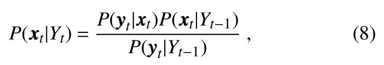
From Eq.(8),we can see that if the relative probability ofgivenis too small–that is,the prediction observation given the analysis state diverges too far from the actual observation–thefinal conditional PDF ofwill also be very small.This means thatis unlikely to be the true state(Anderson and Anderson,1999)–that is,the analysis statecannot be regarded as a reasonable estimate if the value ofis too small.Therefore,we can evaluate the outcome using this perspective.From this point of view,we construct a confidence region based on the observation to calculate the inflation parameter in the EnKF.

3.1.EnCR method

Based on the descriptions above,we introduce a confi-dence region to testify the feasibility of the analysis state.This idea is similar to the quality control method.Quality control is a method that aims at monitoring the extent to which products meet specifications.By monitoring the quality characteristics,the abnormality of a production procedure can be detected quickly and a measure can be taken in time to guarantee that the process is under control(MacGregor and Kourti,1995;Montgomery,2007).Statistical principles are widely used in quality control and,here,we briefly introduce its procedure based on the χ2statistic.

Suppose the quality characteristic isis the corresponding estimated in-control covariance,andis a prespecified value.The control region can be stated as

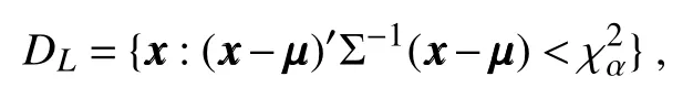
where χαis the α quantile of the χ2distribution.If x x x falls in the region DL,the production process is considered to be normal;otherwise,the process is regarded as out of control and some adjustment procedure needs to be taken.Usually,α is set as 0.99;that is

Similarly,we can view the EnKF method with an unknown adjustment parameter as a production process,and the analysis state can be viewed as the corresponding product of the process.Hence,we can determine the parameter based on the idea of quality control and construct the corresponding control region as follows:First,the product(analysis state)can be expressed as

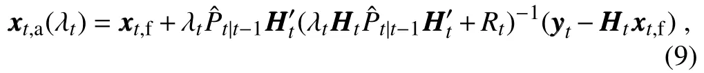
which is controlled by parameter λt,and x x xt,frepresents the prior forecast of the state.The observation can be viewed as the pre-specified value,and the control statistic can be constructed by

where Vtis the in-control covariance matrix that can be calculated by

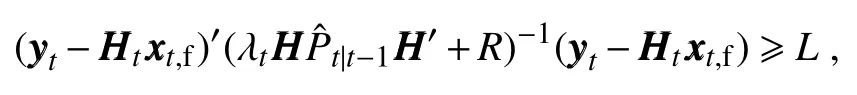
The parameter λtneeds to be adjusted when xxxt,afalls outside the control region(confidence region):

where L is the α quantile of the χ2(n)distribution and is usually set between 0.90 and 0.99,and n is the dimension of yyyt.

Theorem 3.1:Under assumption(7),we have

Theorem 3.2:Under assumption(7),the analysis state variance of EnCR can be expressed as

Theorem 3.3:The control statistic can be expressed as

Based on the results of theorem 3.3,we can ascertain that λtis a monotonically decreasing function of ut(λt);therefore,the adjustment parameter can be constructed by Eqs.(11)and(14).That is,if the initial value λt∉ D,we increase λtuntil it falls in the region D.In this paper,the parameter λtthatfirst falls in region D is used as its estimate.We also note that the calculation of λtin Eq.(14)only involves the dimension of the observation,which is time-saving,especially in some high-dimensional situations,if the dimension of the observation is much smaller than the state.

Next,the algorithm procedure of the EnCR is presented.

3.2.EnCR procedure

Based on the descriptions stated above,the EnCR procedure can be expressed as follows:

(2)Generate the initial ensemblefromand set t=1.

(3)Set the initial parameter λt=1 and calculate the forecast state and its variance by

(4)Iftheinequalitybelowholds,gotostep(5);otherwise,go to step(6):

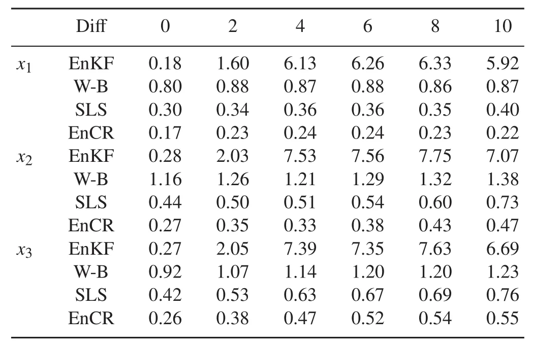
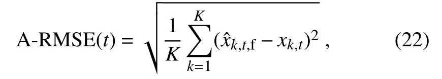
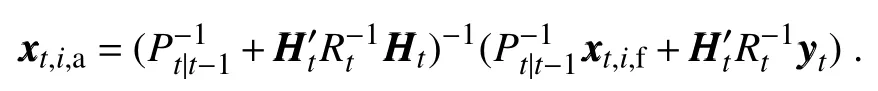
(5)If λt

(6)Generate the observation samples γ1,γ2,...,γmfrom N(0,Rt)and evaluate the analysis ensemble,analysis state and its variance by

(7)If t reaches the last time point,stop the algorithm;otherwise,go to step(3).

Then,the analysis state of all the observation time can be obtained.

4.Experiments on Lorenz models

In this section,we evaluate thefinite sample performance of the EnCR method with the Lorenz-63 and Lorenz-96 models.Both these models have chaotic behavior and are very sensitive to the initial condition settings.In these experiments,some of the model settings are adapted from the work of Evensen(2009)and Wu et al.(2013).To illustrate the performance of the EnCR method,we compare the assimilation results of EnCR with the EnKF,W-B(Wang and Bishop,2003)and SLS methods(Wu et al.,2013).

4.1.Simulation results of the Lorenz-63 model

The Lorenz-63 model is a set of nonlinear differential equations with three variables(Lorenz,1963).The solution of this model has chaotic behavior and is very sensitive to the initial condition settings.Moreover,this model has been examined by various data assimilation methods for their potential applications with other strongly nonlinear and chaotic models,such as oceanic and atmospheric models(Palmer,1993;Anderson and Anderson,1999;Evensen,2009;Sheng and Li,2015).

4.1.1. Forecast model

First,the Lorenz-63 model can be expressed as

where x=(x1,x2,x3)is the state and a,b,c is the model parameter.Here,we adopt the parameter settings of Evensen(2009)and set a=10,b=28,c=8/3.

We use a forecast model with a model error added on model(15):

4.1.2.Observation model

Here,we consider an observation operator whose dimension is less than three:

which is independent of time.

4.1.3. Description of the setup

In this simulation experiment,we set the time step as 0.05 and solve the Lorenz model(15)with a fourth-order Runge–Kutta integration scheme,and the observations are obtained every four time steps.The initial condition is given by=(1,2,3)′,and the true state series are generated by Eq.(16)and denoted by

The observations are generated by Eq.(17)and denoted by yyy0.2, yyy0.4,···, yyy30.We repeat this procedure 200 times and at each time we can obtain an estimate sequence.Hence,the root-mean-square error(RMSE)of the state in the kth dimension of state at time t can be calculated by

wherexk,tis the kth dimension of state at time t;andxk,t,i,fis its ith forecast ensample estimate,where i=1,...,200.For simplicity,we denote RMSEk(t)simply as“RMSE”.It is obvious that a smaller RMSE usually indicates a better performance of the corresponding assimilation method.Moreover,we also use the time-averaged RMSE value as a criterion to compare the performance of different assimilation methods.

4.1.4.Initial condition settings

Since in practical situations the true initial distribution is usuallynotavailable,wesetaninaccurateinitialconditionfor all the assimilation methods in the simulation experiments to study the robustness of the new method.That is,in the numerical experiments of subsection 4.1.5 and subsection 4.1.6,the mean value of the initial distribution used to estimate the state diverges a distance of 10 from the true initial value used to generate the state.The initial distribution is set with a normal distribution with mean(11,12,13)and variance 0.52I3.The ensemble size is 30 in all cases.Additionally,in subsection 4.1.7,the influence of different initial condition settings is further studied via numerical experiments.

4.1.5.Assimilation results of one case

First,we compare the performance of EnCR with the WB and SLS methods in a situation when the model error variance Qt=0.012I3and the observation error variance Rt=I2.

Figure 1 displays the results of the RMSE of the three dimensions of the state based on the W-B,SLS and EnCR methods,separately.From thisfigure,we can see that the convergence rate of the EnCR method is slightly faster than that of the other two methods,and the RMSE values of the SLS and EnCR methods are clearly smaller than that of the W-B method.To further compare the performances of the EnCR and SLS methods,we remove the RMSE line of the W-B method and obtain Fig.2.From thisfigure,it is clear that the EnCR method obtains the smallest RMSE overall.

Moreover,Table 1 demonstrates the time-averaged RMSE values of the EnKF,W-B,SLS and EnCR methods.This table indicates that the W-B,SLS and EnCR methods significantly reduce the time-averaged RMSE of the EnKF method,and the EnCR method achieves the smallest timeaveraged RMSE of all the methods.Furthermore,to study the implications of different variance settings,the four methods are compared under various variance settings in the next subsection.

4.1.6.Implications ofthe modeland observationerrorvariance settings

In this subsection,we study the estimated accuracy and stability of the EnCR method under different error variance settings.

Table 1.Time-averaged RMSE values of different methods.

Fig.1.RMSE of the W–B,SLS and EnCR methods.

Fig.2.RMSE of the SLS and EnCR methods.

First,the observation error variance is set asand the value of model error variance is set aswhere σ1is a varying parameter.The results are demonstrated in Table 2.From this table,we can see that as σ1increases,the estimated precision of all the methods decreases,which is consistent with our intuition.Whenthe time-averaged RMSEs of the SLS and EnCR methods are quite close;and whenthe EnCR method obtains the smallest time-averaged RMSE.Moreover,when the model error variance is large,i.e.the last several columns of Table2,thetime-averagedRMSEoftheW-B,SLSandEnCRmethods are much smaller than that of the EnKF method,and the EnCR method maintains the smallest time-averaged RMSE value,which suggests that the estimated accuracy of the EnCR method is better than that of the other methods.

Table 2.Time-averaged RMSE values of three states in the Lorenz-63 model with a variation of σ1,where Rt=0.12I3and Qt=

Table 2.Time-averaged RMSE values of three states in the Lorenz-63 model with a variation of σ1,where Rt=0.12I3and Qt=

?

Using the information provided in Table 3,we study the influence of the observation error variance when the model error variance isfixed.That is,we set the model error variance Qt=0.12I3and the observation error variancewith different σ2values.From this table,we can see that,overall,the estimated precision of the EnCR method is better than that of the other methods.Moreover,it is also notable that,even when the observation variance is relatively large,the new method performs better than the other three methods.Overall,Table 3 shows that the performance of the new method is significantly superior to the other three methods.

Based on the above results,the estimation results of the EnCR method are superior to the other three methods,particularly when the model error variance is large.Furthermore,as the error variance increases,the estimation precision of all the methods decreases.In short,the simulation results indicate that the new method has a higher estimation precision and is more stable than the other methods.

4.1.7.Implications of the initial condition settings

In this section,the implications of the initial condition settings are examined for different assimilation methods.Here,we set the model error variance Qtto 0.012I3and the observation error variance to Rt=I2.For description simplic-ity,the variance of the initial condition is set to 0.5I3,and we set the same deviation for the simulation initial value of the three state components to the true initial value and denote it by Diff–that is,whereandare the simulation initial state and the true state of x0in the ith component,respectively.

Table 4 gives the estimation results of all the methods under different deviation Diff settings.The time-averaged RMSE of the EnKF method increases significantly as the deviation increases.However,the time-averaged RMSE of the W-B,SLS and EnCR methods grows very slowly as the bias of the model initial condition increases,which indicates that the three methods are not extremely sensitive to the initial condition settings.The estimated precision of the EnCR method is evidently superior to the other methods in this experiment.

It is also interesting to study the estimated inflation values of the three methods with different initial condition settings.As we know,the initial state is biased and the variance in-flation technique should be adopted in thefirst several steps.Here,we consider the mean value of the inflation parameter estimation in thefirst six steps.Table 5 gives the mean value of the inflation parameter with an increase in the bias of theinitial state settings.From this table,we can see that the estimation of the inflation parameter of the new method is more reasonable than the other two methods.That is,when the deviation of the initial state is zero,a smaller inflation should be adopted,and with an increase in the deviation,the inflation parameter should also increase.The inflation estimation of the W-B method is always very large,and the variation of the SLS method is not as reasonable as the new method.

Table 3.Time-averaged RMSE values of three states in the Lorenz-63 model with a variation of σ2,where Rt= and Qt=

Table 3.Time-averaged RMSE values of three states in the Lorenz-63 model with a variation of σ2,where Rt= and Qt=

?

Table 4.Time-averaged values of the RMSE of the three states of the Lorenz-63 model with different initial settings.

Table 5.Time-averaged values of the RMSE of the three states of the Lorenz-63 model with different initial settings.

4.2.Simulation results of the Lorenz-96 model

TheLorenz-96 modelisa 40-dimension differentialequations model,and it is widely used in various data assimilation studies.In this section,we use this model to study the performance of the EnCR method.

4.2.1.Model description and parameter settings

The Lorenz-96 model can be expressed by

where k=1,2,...,K(K=40)and the boundary conditions are assumed to be cyclic;that is,X−1=XK−1,X0=XK,XK+1=X1.Here,F is the external forcing term and we set it to F=8 to generate the true state values in this experiment.The solution of the Lorenz-96 model has chaotic behavior and mimics the temporal evolution of a scalar meteorological quantity on a circle of latitude,and the three terms of the right-hand side of Eq.(19)can be viewed as an advectionlike term,a damping term and an external forcing term,respectively(Wu et al.,2013).Besides,similar to the Lorenz63 model,we use the fourth-order Runge–Kutta time integration scheme to solve the state model(19),and set a time step of 0.05 non-dimensional units to drive the true state.Besides,assuming the characteristic time scale of the dissipation in the atmosphere isfive days,the time step here is roughly equivalent to six hours in real time(Lorenz,1996).

In this model,we adopt the parameter settingsof Wuetal.(2013)and set X0,k=F,k≠20,X0.20=1.01F,with the time step set as 0.2.To achieve stationary estimation results,we obtain the observations every four time steps over a duration of 100 000.

In this study,the observations are generated by an identical observation operator with a Gaussian distribution error:

where the observation error variance Rtis spatially correlated with in which we set σ0=1.

In this study,we use the average state estimate error to compare the performance of different methods,and denote it as A-RMSE:

where K is the dimension of state,xk,tis the true state of the kth dimension at time t,andˆxk,t,fis the corresponding forecast ensemble estimate.Similar to the RMSE criterion,a smaller A-RMSE usually indicates a better performance of the corresponding assimilation method.

4.2.2. Results when F is correctly specified

First,we consider a situation when the forcing term F is correctly specified–that is,there has no model error when estimating the state.Here,we use a normal distribution to generate the initial ensemble:

Figure 3 shows the results of the A-RMSE value of the four methods when the sample size is 20.To make the results clearer,only the A-RMSE results of thefirst 100 s(500 steps)are displayed in thefigure(the trend of A-RMSE after 100 s is similar to the trend around the 100 s).When the sample size is small,the EnCR method obtains the best estimation results,followed by the W-B method.However,the results of the SLS and EnKF methods to a certain degree show up the phenomenon offilter degeneracy in this case.

Figure 4 presents the results of the A-RMSE value when the sample size is 80.In this case,the EnKF method relievesthephenomenonoffilterdegeneracyintheinitialstage.However,over time,the EnKF method begins to degenerate at approximately 15 s.Overall,the other three methods prevent thefilter degeneration phenomenon quite well,and the estimated accuracy of the SLS and EnCR methods is slightly better than that of the W-B method.

Additionally,Table 6 provides the results of the timeaveraged A-RMSE over 100 000 time steps for all the methods under different sample size settings.Overall,the ARMSE of the EnCR method is smaller and more stable than that of the other methods.Moreover,the estimation results of the EnKF method are the poorest,which is coincident with our intuition.

Fig.3.A-RMSE value of the EnKF,W-B,SLS and EnCR methods when the sample size is 20.

Fig.4.A-RMSE value of the EnKF,W-B,SLS and EnCR methods when the sample size is 80.

Table 6.Time-averaged value of A-RMSE over 100 000 time steps of the EnKF,W-B,SLS and EnCR methods under different sample size settings.

4.2.3.Results when F is incorrectly specified

Since the true model is usually not available,a model used in practical situations is always an approximation of the real one.Therefore,studying the estimation performance of a data assimilation method in the situation when the model is incorrectly specified is meaningful.Here,we also use the A-RMSE criterion to examine the estimation robustness of different models.

We also adopt the model parameter settings in subsection 4.2.2 and set F=8 to generate the true states;however,we use different values of F when we estimate the states,such as F=4,5,...,12.

Figure 5 shows the results of the time-averaged A-RMSE over 100 000 time steps of the four methods with different forcing term values when the sample size is 20.When the sample size is small,the time-averaged A-RMSE of the EnCR method is smallest among all methods.Moreover,the time-averaged A-RMSE values of the SLS and EnKF methods are significantly larger than those of the other two methods.It is also very interesting that the minimum value of the time-averaged A-RMSE of the SLS and EnKF methods is not achieved at the point when F=8,in which the value of F is same with that of the model when we generate the data.This is a little inconsistent with our intuition and is possibly because when the sample size is very small,both methods are degenerated(as shown in Fig.3),and thus the observation information contributes very little to the state estimation process.Next,we verify this conjecture by increasing the sample size in the following simulations.

Fig.5.Time-averaged A-RMSE over 100 000 time steps of the four methods for different settings of the forcing term F when the sample size is 20.

Fig.6.Time-averaged A-RMSE over 100 000 time steps of the four methods for different settings of the forcing term F when the sample size is 80.

Fig.7.Time-averaged A-RMSE over 100 000 time steps of the four methods for different settings of the forcing term F when the sample size is 100.

Figures 6–7 show the results when the sample size is 80 and 100,respectively.First,we can see that when the sample size is large,the EnKF and SLS methods achieve their minimum time-averaged A-RMSE when F=8,which verifies the above conjecture.When F is around the true value,there has very little difference in estimation among the SLS,W-B and EnCRmethods.However,when F ismuchsmallerthan8,the W-B method achieves the smallest time-averaged A-RMSE,but the results of the EnCR and W-B methods are almost indistinguishable.When F is much larger than 8,the EnCR method achieves the best precision among all the methods.Based on the above results,we can conclude that the EnCR method demonstrates preferable performance and robust estimation results compared with the other methods.

4.3.Summary of the experimental results

From the experiments using the Lorenz-63 model,we can draw the following conclusions:

(1)Overall,the EnCR method performs best.The SLS method ranks second and,when the observation error variance is small,the precision values of the SLS and EnCR methods are very close.However,when the observation error variance is large,the performance of the EnCR method is clearly better than the other methods.

(2)With the model error variance increases,the precision of the EnCR and SLS methods tends to be similar and better than that of the W-B and EnKF methods.

(3)The EnCR,W-B and SLS methods are not very sensitive to the initial condition settings,and the estimation results of the EnCR method are better than those of the other two methods under different initial deviation settings,which suggests the new method produces a more robust and highly precise estimation result.

From the experiments using the Lorenz-96 model,we can draw the following conclusions:

(1)When the model forcing parameter is correctly speci-fied and the sample size is small,the EnCR method is better than the other methods.With the sample size increases,the precision values of the W-B,SLS and EnCR methods become very close to one another.

(2)Whenthemodelforcingparameterisincorrectlyspecified,the EnCR method is better than the other methods when the sample size is small.When F used in the model is smaller than the true value and the sample size is large,the W-B method obtains the best results,and the results of the EnCR method are very close to the results of the W-B method in that case.Moreover,when F is larger than the true value,the EnCR method achieves the best results and is clearly better than the other methods.

5.Conclusions

In this paper,we propose a new method to estimate the forecast error variance inflation parameter in the classical EnKF method.In the simulation experiments,the new method significantly improves the accuracy of the EnKF method and achieves robust estimation results when the initial settings and model parameters are incorrectly specified.Moreover,basedonoursimulationprocess,whentheforecast model or the initial settings are very poor,the adjustment parameter estimated by the new method can be very large,and in this situation the observation information is fully used to obtain a robust estimate.Therefore,the parameter estimate of the new method is moreflexible than the other methods.However,although the new method performs quite well in the simulations,when dealing with high-dimensional problems the inverse of λtHˆPt|t−1H′+Rtin the algorithm will be expensive if the dimension of the observation is also very high.In this case,our conjecture that some diagonal substitution of λtHˆPt|t−1H′+Rtcould possibly be adopted to save on computation time if λtHˆRt|t−1H′+Rtis diagonal dominant.We intend to consider the situation of a high-dimensional case in future research.

Using the idea of a confidence region to estimate the parameter of the EnKF method can also be extended to other unknown parameter estimation problems within data assimilation methods.In our future studies,the idea of a confidence region will be further studied in a similar direction.

Acknowledgements.This work was supported in part by the National Key Basic Research Development Program of China(Grant No.2010CB950703),the Fundamental Research Funds for the Central Universities of China and the Program of China Scholarships Council(CSC No.201506040130).The authors are very grateful to the Editor,the Editorial Office,and the two reviewers,for their many insightful comments and helpful advice,which led to a substantially improved manuscript.

APPENDIX

Proof of Theorem 1

From Eq.(9)we can obtain

Then,from Eqs.(6)and(7),

This completes the proof.

Proof of Theorem 2

From Eq.(4),xtsatisfies the linear regression model below:

Notice that:

The results of Theorem 2 can then be achieved by assumption(7).

Proof of Theorem 3

Then,substituting the above equation into the expression of the statistic,we obtain

This completes the proof of Theorem 3.

Anderson,J.L.,and S.L.Anderson,1999:A Monte Carlo implementation of the nonlinearfiltering problem to produce ensemble assimilations and forecasts.Mon.Wea.Rev.,127(12),2741–2758,https://doi.org/10.1175/1520-0493(1999)127<2741:AMCIOT>2.0.CO;2.

Burgers,G.,P.Jan van Leeuwen,and Evensen,G.,1998:Analysis scheme in the ensemble Kalmanfilter.Mon.Wea.Rev.,126(6),1719–1724,https://doi.org/10.1175/1520-0493(1998)126<1719:ASITEK>2.0.CO;2.

Chan,Y.T.,A.G.C.Hu,and J.B.Plant,1979:A Kalmanfilter based tracking scheme with input estimation.IEEE Transactions on Aerospace and Electronic Systems,AES-15,237–244,https://doi.org/10.1109/TAES.1979.308710.

Evensen,G.,1994:Sequential data assimilation with a nonlinear quasi-geostrophic model using Monte Carlo methods to forecast error statistics.J.Geophys.Res.:Oceans,99(C5),10 143–10 162,https://doi.org/10.1029/94JC00572.

Evensen,G.,2009:Data Assimilation:The Ensemble Kalman Filter.2nd ed.Springer Science&Business Media,307 pp.

Gordon,N.J.,D.J.Salmond,and A.F.M.Smith,1993:Novel approach to nonlinear/non-Gaussian Bayesian state estimation.IEEE Proceedings F:Radar and Signal Processing,140(2),107–113,https://doi.org/10.1049/ip-f-2.1993.0015.

Houtekamer,P.L.,and H.L.Mitchell,2001:A sequential ensemble Kalmanfilter for atmospheric data assimilation.Mon.Wea.Rev.,129(1),123–137,https://doi.org/10.1175/1520-0493(2001)129<0123:ASEKFF>2.0.CO;2.

Kalman,R.E.,1960:A new approach to linearfiltering and prediction problems.Journal of Basic Engineering,82(1),35–45,https://doi.org/10.1115/1.3662552.

Li,H.,E.Kalnay,and T.Miyoshi,2009:Simultaneous estimation of covariance inflation and observation errors within an ensemble Kalmanfilter.Quart.J.Roy.Meteor.Soc.,135(639),523–533,https://doi.org/10.1002/qj.371.

Linderoth,M.,K.Soltesz,A.Robertsson,and R.Johansson,2011:Initialization of the Kalmanfilter without assumptions on the initial state.Proc.2011 IEEE International Conference on Robotics and Automation,Shanghai,China,IEEE,4992–4997,https://doi.org/10.1109/ICRA.2011.5979684.

Lorenc,A.C.,2003:The potential of the ensemble Kalmanfilter for NWP–a comparison with 4D-Var.Quart.J.Roy.Meteor.Soc.,129(595),3183–3203,https://doi.org/10.1256/qj.02.132.

Lorenz,E.N.,1963:Deterministic nonperiodicflow.J.Atmos.Sci.,20(2),130–141,https://doi.org/10.1175/1520-0469(1963)020<0130:DNF>2.0.CO;2.

Lorenz,E.N.,1996:Predictability–A problem partly solved.Proc.Seminar on Predictability,ECMWF,Shinfield Park,Reading,Berkshire,UK,ECMWF.

MacGregor,J.F.,and T.Kourti,1995:Statistical process control of multivariate processes.Control Engineering Practice,3(3),403–414,https://doi.org/10.1016/0967-0661(95)00014-L.

Montgomery,D.C.,2007:Introduction to Statistical Quality Control.John Wiley&Sons,734 pp

Palmer,T.N.,1993:Extended-range atmospheric prediction and the Lorenz model.Bull.Amer.Meteor.Soc.,74(1),49–65,https://doi.org/10.1175/1520-0477(1993)074<0049:ERAPAT>2.0.CO;2.

Salmond,D.,and N.Gordon,2005:An introduction to particlefilters.State Space and Unobserved Component Models Theory and Applications,1–19

Sheng,Y.,and Y.Li,2015:An ensemble forecast method based on observational errors.Journal of Beijing Normal University(Natural Science),2015(1),9–13,https://doi.org/10.16360/j.cnki.jbnuns.2015.01.003.(in Chinese)

van Loon,M.,P.J.Builtjes,and A.J.Segers,2000:Data assimilation of ozone in the atmospheric transport chemistry model LOTOS.Environmental Modelling&Software,15(6),603–609,https://doi.org/10.1016/S1364-8152(00)00048-7.

Wang,X.G.,and C.H.Bishop,2003:A comparison of breeding and ensemble transform Kalmanfilter ensemble forecast schemes.J.Atmos.Sci.,60(9),1140–1158,https://doi.org/10.1175/1520-0469(2003)060<1140:ACOBAE>2.0.CO;2.

Wang,Y.,M.Bellus,J.F.Geleyn,X.L.Ma,W.H.Tian,and F.Weidle,2014:A new method for generating initial condi-tion perturbations in a regional ensemble prediction system:Blending.Mon.Wea.Rev.,142(5),2043–2059,https://doi.org/10.1175/MWR-D-12-00354.1.

Welch,G.,and G.Bishop,1995:An introduction to the Kalmanfilter.Tech.Rep.,Department of Computer Science,University of North Carolina at Chapel Hill Chapel Hill,NC,USA.Wu,G.C.,X.G.Zheng,L.Q.Wang,S.P.Zhang,X.Liang,and Y.Li,2013:A new structure for error covariance matrices and their adaptive estimation in EnKF assimilation.Quart.J.Roy.Meteor.Soc.,139(672),795–804,https://doi.org/10.1002/qj.2000.

Zheng,H.,and Coauthors,2015:A global carbon assimilation system based on a dual optimization method.Biogeosciences,12(4),1131–1150,https://doi.org/10.5194/bg-12-1131-2015.