基于空间自相关的天然蒙古栎阔叶混交林林木胸径-树高模型*

娄明华 张会儒 雷相东 李春明 臧 颢

(1.中国林业科学研究院资源信息研究所 北京 100091; 2.宁波市农业科学研究院 宁波 315040; 3.江西农业大学林学院 南昌 330045)



基于空间自相关的天然蒙古栎阔叶混交林林木胸径-树高模型*

娄明华1,2张会儒1雷相东1李春明1臧 颢3

(1.中国林业科学研究院资源信息研究所 北京 100091; 2.宁波市农业科学研究院 宁波 315040; 3.江西农业大学林学院 南昌 330045)

【目的】 考虑林木间的空间自相关，构建基于空间自相关的林木胸径-树高模型，为可持续经营天然混交林提供理论依据。【方法】 以天然蒙古栎阔叶混交林为研究对象，选择适宜的线性化林木胸径-树高模型为基础模型(BM)，应用3个同步自回归(SAR)模型即空间滞后模型(SLM)、空间误差模型(SEM)和空间Durbin模型(SDM)研究该混交林的林木胸径-树高模型。同时，将Delaunay三角网(DT)矩阵、逆距离一次幂(ID1)、逆距离二次幂(ID2)、逆距离五次幂(ID5)、球状变异函数(SV)矩阵、高斯变异函数(GV)矩阵和指数变异函数(EV)矩阵共7个空间加权矩阵应用于SAR模型中。利用普通最小二乘法(OLS)估计BM参数，极大似然法估计3个SAR模型参数，并对4个模型的回归参数进行T检验，对3个SAR模型的自回归参数进行似然比检验。选择Moran’s I(MI)指数比较分析BM、SLM、SDM和SEM 4个模型的残差空间自相关，选择决定系数(R2)、均方根误差(RMSE)和Akaike信息准则(AIC)3个拟合指标比较分析4个模型的拟合效果。【结果】 空间加权矩阵SV的BM残差MI值大于1，因此以下结果分析中将不再考虑SV。其他6个空间加权矩阵的BM和SLM残差MI值均显著大于期望值I0，但SLM残差MI值较相同空间加权矩阵的BM残差MI值小。除了GV和ID1外，其他4个空间加权矩阵的SDM残差MI值均与I0差异不显著。除了ID1外，其他5个空间加权矩阵的SEM残差MI值均与I0差异不显著。3个SAR模型的3个拟合指标均优于BM。在相同的空间加权矩阵中，SDM和SEM的3个拟合指标非常接近，但均优于SLM。在SDM和SEM中，不同空间加权矩阵(除GV外)根据3个拟合指标从优至劣的排序为ID2> DT > ID > ID5 > EV。无论采用哪个空间加权矩阵，3个SAR模型的回归参数β1均与BM中的β1相似，且均显著不为零。相比β1，SEM和BM中的β0相似，但SDM和SLM中的β0与BM中的β0不相似，并且随着空间加权矩阵的变化而变化。应用于SAR模型的所有空间加权矩阵中，利用ID1得出的自回归参数ρ、γ和λ均明显高于利用其他空间加权矩阵计算的值。GV只有在SEM中才能使自回归参数λ显著。除了GV外，利用其他5个空间加权矩阵得出的ρ、γ和λ均显著。【结论】 应用于SAR模型的7个空间加权矩阵中，SV和ID1为不合理的空间加权矩阵。SLM只能降低模型残差的空间自相关，改善模型拟合效果较SDM和SEM差。只要选择合适的空间加权矩阵，SDM和SEM就可以消除模型残差的空间自相关，提高模型拟合效果，其中ID2是最好的空间加权矩阵。利用ID2和SEM构建以树种为哑变量的胸径-树高模型，从而得出基于空间自相关的蒙古栎、杨桦(山杨和白桦)、红松的胸径-树高模型。关键词： 空间自相关； 胸径； 树高； 自回归模型； 空间滞后

Individual Diameter-Height Models for MixedQuercus

胸径和树高是森林调查及经营管理的2个重要因子(Leietal., 2009)。相对于胸径，树高的测量比较困难，存在成本高、耗时长、观测误差大、视觉阻碍(如树梢顶部容易遮挡，特别是天然混交林)等不利因素(Chhetrietal., 1996; Colbertetal., 2002; Mehtätalo, 2004; Trincadoetal., 2007; Krisnawatietal., 2010; Sharmaetal., 2015)，因此，学者们经常利用林木胸径-树高模型估计树高，进而估计林木材积、立地质量、林分动态以及其他有关森林生长与收获(Leietal., 2001; Peng, 2001; Calamaetal., 2004; Leietal., 2009)。

传统林木胸径-树高模型均假定林木间是相互独立的，通常采用普通最小二乘法(ordinary least squares, OLS)进行估计。然而，随着研究的逐步深入，学者们逐渐意识到林木间的关系并不是相互独立的(Frodetal., 1981; Tomppo, 1986; Mateuetal., 1998)，这是因为林木间的竞争和微环境结合作用，导致林木间存在空间自相关(spatial autocorrelaton)(Magnussen, 1990; Foxetal., 2001)。空间自相关是指一些变量在同一分布区内的观测数据之间潜在的相互依赖性，一般认为，相邻林木间的空间自相关程度强于相离林木间的空间自相关程度(Legendre, 1993; Legendreetal., 1998),因此，忽略空间自相关将会使OLS回归违背残差独立分布假设，导致犯第一类错误(原假设为真，假设检验拒绝了原假设)的可能性变大(Legendre, 1993; Lennon, 2000; Legendreetal., 2002; Dormannetal., 2007; Kisslingetal., 2008)、模型参数标准差的有偏估计及回归模型估计有效性降低(Krämer, 1980; Westetal., 1984; Gregoire, 1987; Foxetal., 2001; Zhangetal., 2004b)等。

鉴于林木间存在空间自相关，目前已有学者将空间自相关模型加入到林木胸径-树高模型中，如地理加权回归(geographically weighted regression)模型(Zhangetal., 2004a; 2004b; 2005)、同步自回归(simultaneous autoregressive, SAR)模型(Mengetal., 2009; Luetal., 2011)等，其中，SAR模型全面考虑了空间自相关过程发生在模型应变量、模型解释变量及模型误差中的可能性，是常用的空间自相关模型(Kisslingetal., 2008; Mengetal., 2009; Luetal., 2011)。具体来说，SAR模型包括空间滞后模型(spatial lag model, SLM)、空间误差模型(spatial error model, SEM)和空间Durbin模型(spatial Durbin model, SDM)，SLM假设空间自回归过程只发生在应变量中，SEM假设该过程只发生在模型误差项中，SDM假设该过程同时发生在应变量和解释变量中(Cressie, 1993; Haining, 2003)。

蒙古栎(Quercusmongolica)阔叶混交林是我国东北地区主要的天然次生林，蒙古栎主干坚硬耐腐、纹理美观，是良好的造材原料，枝条发热量高，可作为良好的薪炭材，叶可饲蚕和动物，根系发达且适应性强，具有涵养水源、 防风固沙、 减少径流、保持水土等作用，果实富含淀粉，经加工提炼可转化燃料乙醇及生物化工产品(田超等， 2011； 马武， 2012)，对国民经济和生态环境均具有很高的价值(于顺利等， 2001； 2004； 许中旗等， 2006； 陈新美等， 2010； 洪玲霞等， 2012)。为此，本文以天然蒙古栎阔叶混交林为研究对象，考虑林木间的空间自相关，构建基于空间自相关的林木胸径-树高模型，以期为可持续经营天然混交林提供理论依据。

1 材料与方法

1.1 研究区概况与样地调查

研究区位于吉林省汪清林业局塔子沟林场，地理坐标为129.971°—130.222°E，43.327°—43.492°N。属长白山系老爷岭山脉雪岭支脉，低山丘陵地貌，海拔300～1 200 m，坡度5°～25°。研究区属季风性气候，年均气温3.9 ℃左右，年均降水量600～700 mm，且集中在夏季，占全年总降水量的80%。土壤主要以暗棕壤为主，平均厚度40 cm左右。植被属长白山植物区系，群落结构复杂，植物种类较多，主要树种有蒙古栎、白桦(Betulaplatyphylla)、红松(Pinuskoraiensis)、山杨(Populusdavidiana)、榆(Ulmuspumila)、椴(Tiliatuan)、黑桦(Betuladahurica)、长白落叶松(Larixolgensis)、色木槭(Acermono)、红皮云杉(Piceakoraiensis)、冷杉(Abiesfabri)、水曲柳(Fraxinusmandshurica)、黄檗(Phellodendronamurense)等。

2013年7—9月，在塔子沟林场选择典型的天然蒙古栎阔叶混交林，设置100 m×100 m固定样地，样地坡度8°，坡位为中坡，坡向为西坡，样地中心海拔705 m，样地左下角坐标为130.112°E，43.450°N。利用森林罗盘仪，将样地划分100个10 m×10 m的网格单元，在每个网格单元内对胸径5 cm以上的树木进行每木调查，记录树种，测量胸径、树高、枝下高、东西南北冠幅等因子，并利用徕卡激光测距仪测定林木坐标(X，Y)。样地林分特征详见表1。

1.2 基础林木胸径-树高模型

由表1可知，天然蒙古栎阔叶混交林中有4个主要树种，即蒙古栎、白桦、红松和山杨。考虑到山杨和白桦具有相近的林木生长特性，本文将山杨和白桦称为杨桦，作为同一建模树种，并建立全林分、蒙古栎、杨桦和红松4个胸径-树高模型。为不改变林木间的空间关系即林木间的空间自相关结构，采用哑变量方法即以树种为哑变量构建分树种的胸径-树高模型(简称哑变量模型)。

当前SAR模型均为线性的(Mengetal., 2009)，因此本文只考虑线性化的基础林木胸径-树高模型。根据图1所示的胸径与树高散点图，选用3个备选线性化基础模型，具体见表2。

1.3 同步自回归模型

SAR模型包括空间滞后模型(SLM)、空间误差模型(SEM)和空间Durbin模型(SDM)，其表达式(Cliffetal., 1981; Anselin, 1988; Haining, 2003; Fortinetal., 2005; Dormannetal., 2007)如下：

(1)

(2)

(3)

式中：Y表示应变量矩阵；X表示解释变量矩阵；W表示空间加权矩阵；β表示回归系数；ε表示模型残差；ρ、λ和γ表示空间自回归系数；ξ表示空间相关残差。

表1 固定样地林分特征①Tab.1 Stand characteristics of permanent plots

①N表示林木株数； BA表示断面积； SBA表示树种断面积比例；Dmean、Dmax和Dmin分别表示平均胸径、最大胸径和最小胸径；Hmean、Hmax和Hmin分别表示平均树高、最大树高和最小树高。Ndenote tree number; BA denote basal area; SBA denote species basal area ratio;Dmean,DminandDmaxdenote mean, minimum and maximum diameter at breast height;Hmean,HminandHmaxdenote mean, minimum and maximum tree height.

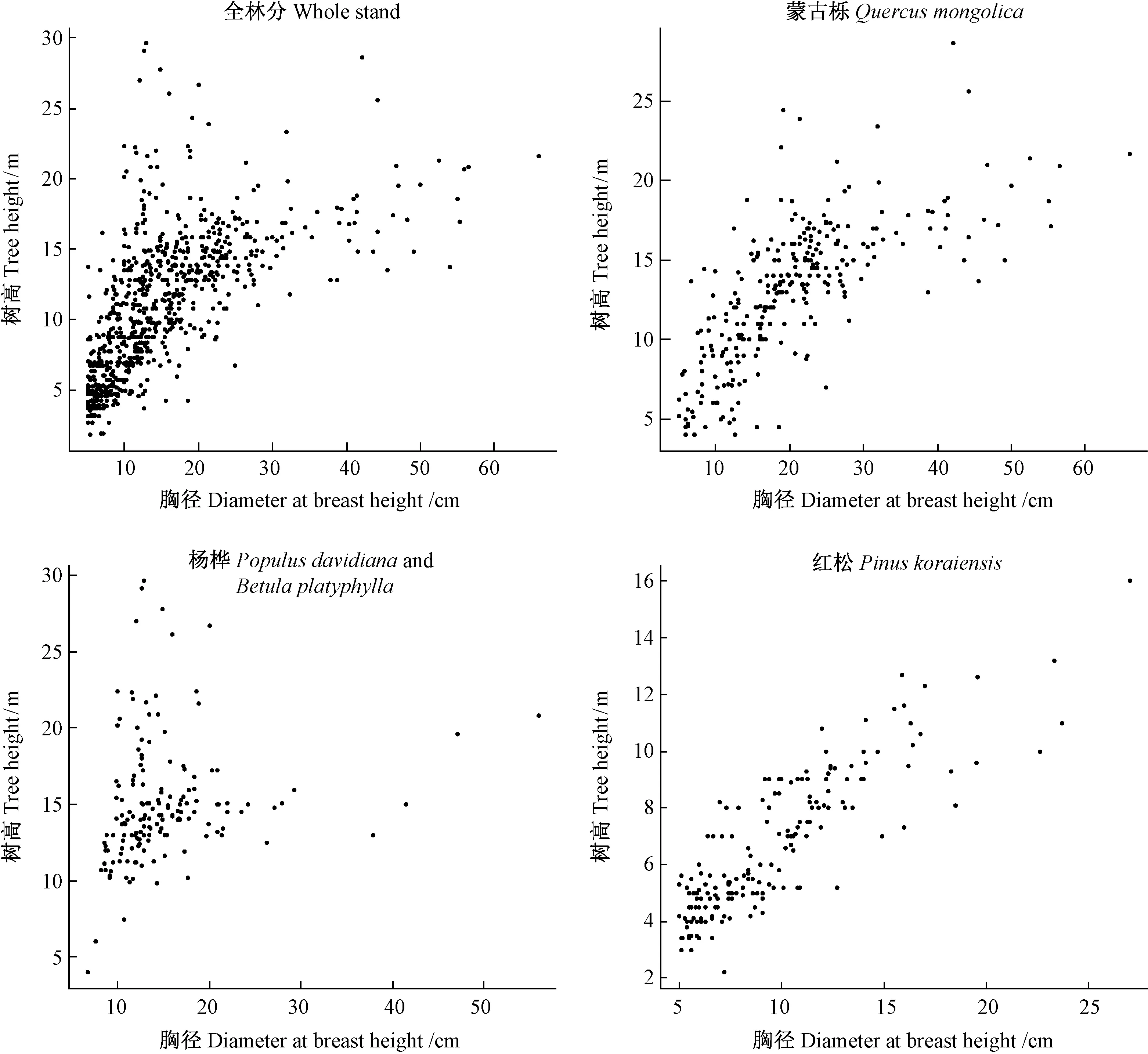
图1 不同树种的胸径-树高散点示意Fig.1 Scatter plot of diameter at breast height against tree height for different species

模型序号ModelNo．模型表达式Modelexpression参考文献ReferencesAlnH=β0+β1lnD+εCurtis，1967BlnH=β0+β1D+εHuangetal．，1992；李希菲等，1994．ClnH=β0+β1D-1+εCurtis，1967

①H表示树高；D表示胸径；β0和β1表示回归系数；ε表示模型残差。Hdenotes tree height;Ddenotes diameter at breast height;β0andβ1denote regression coefficients;εdenotes model error term.

WY、WX和Wξ为3个空间滞后变量。当ρ=0时，式(1)变为线性回归模型； 当λ=0时，式(2)变为线性回归模型； 当ρ和γ同时为零时，式(3)变为线性回归模型。采用极大似然法(maximum likelihood)估计3个SAR模型的参数，通过R统计语言spdep包的lagsarlm和errorsarlm函数实现。

1.4 空间加权矩阵

空间加权矩阵(spatial weight matrix)是SAR模型的重要组成部分，本文选取常用的空间加权矩阵，即相接邻近(contiguous neighbors)矩阵、逆距离幂(inverse distances raised to some power)矩阵和地统计(geostatistical)矩阵(Getisetal., 2004; Luetal., 2011)。

相接邻近矩阵包括Rook相接矩阵、Queen相接矩阵、Bishop相接矩阵(Anselin, 2001)和Delaunay三角网(Delaunay triangulation, DT)矩阵(Smirnovetal., 2001)等。其中，Rook相接矩阵、Queen相接矩阵和Bishop相接矩阵一般用于规则的空间相接关系，DT矩阵可处理不规则的空间相接关系，因为林木间的空间关系一般是不规则的，因此本文采用DT矩阵。DT矩阵中，林木间为相接邻近关系时，其空间加权值为1；否则为0。同时，利用R统计语言spdep包的trib2nb函数计算空间加权值。

逆距离幂矩阵包括逆距离一次幂(inverse distances raised to one power, ID1)、逆距离二次幂(inverse distances raised to two power, ID2)和逆距离五次幂(inverse distances raised to five power, ID5)3种形式(Getisetal., 2004)，其表达式如下：

(4)

式中：dij表示林木i与其相邻木j的距离，wij表示林木i与其相邻木j的空间加权值，当n=1时，则为ID1； 当n=2时，则为ID2； 当n=5时，则为ID5。

Getis等(2004)利用满足本征假设(intrinsic stationarity)的变异函数构建了3个地统计矩阵，即球状变异函数(spherical variogram, SV)矩阵、高斯变异函数(Gaussian variogram, GV)矩阵和指数变异函数(exponential variogram, EV)矩阵，其表达式如下：

(5)

(6)

(7)

式中：r表示变程，wij和dij意义同上。

利用R统计语言nlme包的corExp、corGaus和corSpher函数分别计算SV、GV和EV矩阵的空间加权值。

本文采用DT、ID1、ID2、ID5、SV、GV和EV共7个空间加权矩阵，应用于3个SAR模型中。

1.5 空间自相关检验指标

选择常用的Moran’s I(MI)指数检验模型残差的空间自相关，其表达式(Paradis, 2014)如下：

(8)

其原假设为I等于期望值I0=-1/(n-1)，表明不存在空间自相关。如果I显著(α=0.01)大于I0，则模型残差为正自相关，说明相邻林木间的相似程度高； 反之如果I显著(α=0.01)小于I0，则模型残差为负自相关，说明相邻林木间的不相似程度高。利用R统计语言spdep包的moran.test函数进行检验。1.6 模型拟合指标

为便于比较模型之间的拟合程度，本文选用决定系数(coefficient of determination,R2)、均方根误差(root mean square error, RMSE)和Akaike信息准则(Akaike information criterion, AIC)3个拟合指标比较分析模型的拟合效果。

2 模型比较分析

从3个备选模型中选择全林分模型和哑变量模型建模效果均最优的线性化基础模型作为全林分和哑变量的基础模型(base model, BM)。值得注意的是，全林分模型和哑变量模型中林木间的空间关系是一致的，即林木间具有一致的空间自相关结构，因此，只需建立基于全林分基础模型的SLM、SEM和SDM共3个SAR模型，并通过比较分析模型残差空间自相关、模型拟合及模型参数估计效果，即可找到最适宜的SAR模型。最后，利用最适宜的SAR模型构建哑变量SAR模型。

2.1 基础模型的确定

利用3个拟合指标R2、RMSE和AIC，分别比较全林分和哑变量模型的3个备选基础模型。由表3可知，全林分模型的备选基础模型C具有最大的R2、最小的RMSE和AIC；哑变量模型的备选模型A具有最大的R2、最小的RMSE和AIC，模型C略低于模型A，最差为模型B。由表4可知，哑变量模型的备选模型A中主要树种蒙古栎和杨桦的参数β0和β1均显著(P<0.01)，主要树种红松的参数β0显著(P<0.01)，而参数β0不显著(P>0.1)。因此，本文选用模型C作为全林分和哑变量的基础胸径-树高模型(BM)。

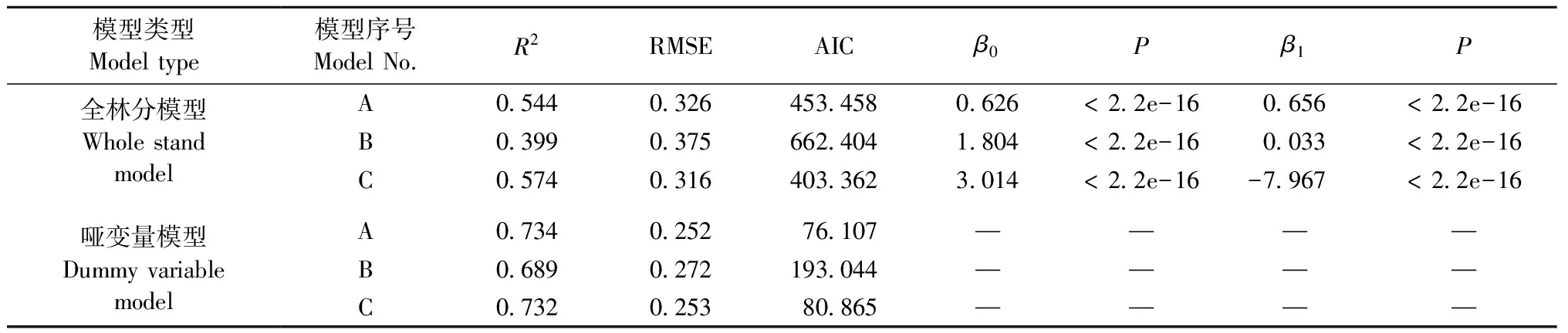
表3 3个备选基础模型的拟合指标及参数估计①Tab. 3 Fitting index and parameter estimates for three alternative base models

①R2：决定系数Coefficient of determination;RMSE:均方根误差Root mean square error;AIC:Akaike信息准则Akaike information criterion.下同The same below.

表4 哑变量模型中3个主要树种的参数估计Tab. 4 Parameter estimates for three main species in dummy variable model

2.2 全林分模型残差空间自相关

由表5可知，空间加权矩阵SV的BM残差MI值大于1，说明SV是不合理的空间加权矩阵，因此，以下结果分析中将不再考虑SV。除了SV外，其他6个空间加权矩阵的BM残差MI值均显著(P< 0.01)大于期望值I0=-1/(752-1)=-0.001 3，说明BM残差存在正空间自相关。6个空间加权矩阵的SLM残差MI值均显著(P< 0.01)大于I0，说明SLM没有消除模型残差的空间自相关，但是降低了空间自相关影响，因其MI值小于相对应的BM残差MI值。除了GV和ID1外，其他4个空间加权矩阵的SDM残差MI值均与I0差异不显著(P> 0.1)，说明选择合适的空间加权矩阵，SDM可以消除模型残差的空间自相关，同时也表明产生模型残差的空间自相关可能是由滞后变量WY(即相邻加权树高)和滞后变量WX(即相邻加权胸径)共同作用产生的。除了ID1外，其他5个空间加权矩阵的SEM残差MI值均与I0差异不显著(P> 0.1)，说明SEM与SDM类似，在合适的空间加权矩阵条件下，SEM可以消除模型残差的空间自相关，但空间自相关可能是由滞后变量Wξ(即相邻加权未观测的变量)产生的，因为SEM的前提假设是空间自相关过程来源于模型误差。

此外，由表5还可知，SDM和SEM 2个SAR模型均能消除模型残差的空间自相关矩阵中，依据MI值和P值，GV是最好的空间加权矩阵，因其有最大P值，但只对SEM有效，其次为EV和ID5，但ID5略逊于EV，最后为ID2和DT。

表5 4个模型残差的空间自相关①Tab. 5 Test for spatial autocorrelation of four model residuals

① W表示空间加权矩阵。下同。 W denotes spatial weight matrix.The same below.

2.3 全林分模型拟合

利用3个拟合指标R2、RMSE和AIC，比较分析BM与3个SAR模型(SLM、SDM和SEM)的拟合效果。由表6和表3可知，3个SAR模型的R2(0.578，0.669)均大于BM，RMSE和AIC均小于BM，说明3个SAR模型的拟合效果均优于BM。3个SAR模型中，SDM与SEM拟合效果不相上下，且均明显优于SLM，这是因为SLM没有消除模型残差的空间自相关(详见2.2)。另外，空间加权矩阵GV在SDM中的拟合效果明显比SEM差，结合表5可知，这是因为GV在SDM中没有消除模型残差的空间自相关。因此，消除模型残差的空间自相关，有助于改善模型拟合效果。

由表6还可知，依据R2、RMSE和AIC，在SDM和SEM中的空间加权矩阵(不考虑GV)从优至劣排序为： ID2> DT > ID > ID5 > EV。

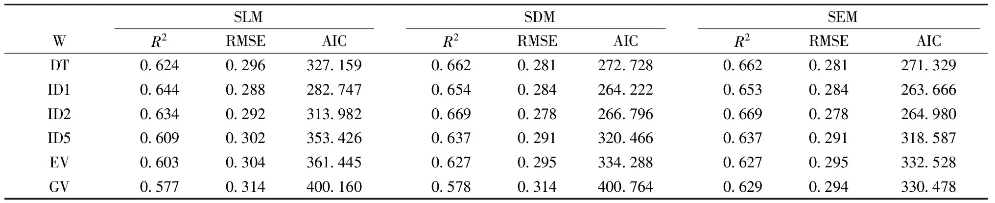
表6 3个SAR模型的拟合Tab. 6 Three SAR models fitting

2.4 全林分模型参数

对3个SAR模型及BM的回归参数进行T检验，对3个SAR模型的自回归参数进行似然比检验(likelihood ratio test)。由表7可知，无论采用哪个空间加权矩阵，3个SAR模型的回归参数β1均与BM中的β1相似，且均显著不为零(P< 2.2e-16)。相比β1，SEM与BM中的β0相似，但SDM和SLM中的β0与BM中的β0不相似，并且随着空间加权矩阵的变化而变化，这主要是由于SDM和SLM的模型形式中增加了空间滞后变量WY和WX。所有的β0中，ID1应用于SDM中的β0与零差异不显著(P>0.1)，说明ID1在SDM中是不理想的空间加权矩阵。同时由表7可知，利用ID1得出的自回归参数ρ、γ和λ均明显高于其他空间加权矩阵得出的值，且无论应用于哪个SAR模型，这进一步说明了ID1是一个不理想的空间加权矩阵。

另外，由表8可知，GV只有在SEM中才能使自回归参数λ显著(P<0.01)。除了GV外，利用其他5个空间加权矩阵得出的ρ、γ和λ均显著(P<0.01)，且均大于零，说明空间滞后变量WY、WX及Wξ均能产生正的空间自相关。

表7 3个SAR模型的回归参数①Tab. 7 Regressive parameters of three SAR models

①BM:β0=3.014,P< 2.2e-16;β1=-7.967,P< 2.2e-16.

表8 3个SAR模型的自回归参数Tab. 8 Autoregressive parameters of three SAR models

2.5 哑变量同步自回归模型

由基于全林分基础模型的SLM、SDM和SEM的残差MI检验效果、建模拟合效果和参数检验效果可知，以ID2为空间加权矩阵的SEM模型是清除基础模型残差空间自相关现象和提高模型精度最佳的同步自回归模型，因此，本文采用该模型建立哑变量SAR模型，得到其R2、RMSE和AIC分别为0.766、0.237和10.728，3个拟合指标均优于哑变量基础模型(表3)，其自回归参数λ为0.412，且显著不为零(P<0.01)。哑变量SAR模型中的蒙古栎、杨桦和红松的参数估计结果见表9。由表9可知，3个主要树种的截距参数β0和β1均显著不为零(P<0.01)，参数检验效果理想。以ID2和SEM建立的全林分SAR模型残差、哑变量SAR模型残差以及3个主要树种的模型残差见图2。

表9 哑变量模型中3个主要树种的参数估计Tab. 9 Parameter estimates for three main species in dummy variable model

图2 不同模型残差Fig.2 Residuals of different models A表示全林分SAR模型； B表示哑变量SAR模型； C表示主要树种蒙古栎； D表示主要树种杨桦； E表示主要树种红松。A denotes whole stand SAR model; B denotes Dummy variable SAR model; C denotes main species of Quercus mongolica; D denotes main species of Populus davidiana and Betula platyphylla; E denotes main species of Pinus koraiensis.

3 结论

本文以线性化林木胸径-树高模型为基础模型(BM)，加入3个SAR模型(SDM、SEM和SLM)构建了基于空间自相关的天然蒙古栎阔叶混交林林木胸径-树高模型，得到以下结论：

1) SDM和SEM能很好地处理空间自相关，而SLM最差，这一结论与Kissling等(2008)、Meng等(2009)和Lu等(2011)研究结果类似。

2) 无论采用哪个空间加权矩阵，SLM均不能消除模型残差空间自相关，但可降低空间自相关，在一定程度上提高了模型拟合效果。

3) 模型残差MI值均与I0差异不显著，SDM和SLM虽能消除模型残差空间自相关，提高模型拟合效果，但需要选择合适的空间加权矩阵，如可选择ID2、DT、ID5和EV，其中ID2最好，能将全林分基础模型的R2从0.574提高到0.669，哑变量基础模型的R2从0.732提高到0.766。

4) 所有7个空间加权矩阵中，SV和ID1应用于胸径-树高模型时，均为不合理的空间加权矩阵。

5) 蒙古栎阔叶混交林林木胸径-树高模型残差的空间自相关可能由滞后变量WY(即相邻加权树高)和WX(即相邻加权胸径)共同产生或者可能由滞后变量Wξ(即相邻加权未观测的变量)产生。

6) 利用ID2和SEM构建了哑变量模型，从而得出蒙古栎、杨桦和红松的同步自回归胸径-树高模型。

本文研究了基于空间自相关的天然蒙古栎阔叶混交林林木胸径-树高模型，得出ID2和SEM是最适宜的空间自相关模型。对于其他林分类型，该模型是否最适宜是下一步需要探讨的问题。另外，本文只构建了基于线性化空间自相关模型的天然蒙古栎阔叶混交林林木胸径-树高模型，如何研究非线性化空间自相关模型就目前来说是一个难题，也是今后的重点研究方向。

陈新美, 张会儒, 姜慧泉. 2010. 东北过伐林区蒙古栎林空间结构分析与评价. 西南林学院学报, 30(6): 20-24.

(Chen X M, Zhang H R, Jiang H Q. 2010. Analysis and evaluation on spatial structure ofQuercusmongolicaforests in over-logged region in northeast China. Journal of Southwest Forestry University, 30(6): 20-24. [in Chinese])

洪玲霞, 雷相东, 李永慈. 2012. 蒙古栎林全林整体生长模型及其应用. 林业科学研究, 25(2): 201-206.

(Hong L X, Lei X D, Li Y C. 2012. Integrated stand growth model of mongolian oak and its application. Forest Research, 25(2): 201-206. [in Chinese])

李希菲, 唐守正, 袁国仁,等. 1994. 自动调控树高曲线和一元立木材积模型. 林业科学研究, 7(5): 512-518.

(Li X F, Tang S Z, Yuan G R,etal. 1994. Self-adjusted height-diameter curves and one entry volume model. Forest Research, 7(5): 512-518. [in Chinese])

马 武. 2012. 蒙古栎林单木生长模型系统. 北京: 中国林业科学研究院硕士学位论文.

(Ma W. 2012. Individual tree growth model system for mongolian oak forest. Beijing: MS thesis of Chinese Academy of Forestry. [in Chinese])

田 超, 杨新兵, 李 军, 等. 2011. 冀北山地不同海拔蒙古栎林枯落物和土壤水文效应. 水土保持学报, 25(4): 221-226.

(Tian C, Yang X B, Li J,etal. 2011. Hydrological effects of forest litters and soil ofQuercusmongolicain the different altitudes of north mountain of Hebei province. Journal of Soil and Water Conservation, 25(4): 221-226. [in Chinese])

许中旗, 李文华, 刘文忠, 等. 2006. 我国东北地区蒙古栎林生物量及生产力的研究. 中国生态农业学报, 14(3): 21-24.

(Xu Z Q, Li W H, Liu W Z,etal. Study on the biomass and productivity of mongolian oak forests in northeast region of China. Chinese Journal of Eco-Agriculture, 14(3): 21-24. [in Chinese])

于顺利, 马克平, 陈灵芝, 等. 2001. 黑龙江省不同地点蒙古栎林生态特点研究. 生态学报, 21(1): 41-46.

(Yu S L, Ma K P, Chen L Z,etal. 2001. The ecological characteristics ofQuercusmongolicaforest in Heilongjiang Province. Acta Ecologica Sinica, 21(1): 41-46. [in Chinese])

于顺利, 马克平, 徐存宝, 等. 2004. 环境梯度下蒙古栎群落的物种多样性特征. 生态学报, 24(12): 2932-2939.

(Yu S L, Ma K P, Xu C B,etal. 2004. The species diversity characteristics comparison ofQuercusmongolicacommunity along environmental gradient factors. Acta Ecologica Sinica, 24(12): 2932-2939. [in Chinese])

Anselin L. 1988. Spatial econometrics: methods and models. Dordrecht: Kluwer Academic Publishers.

Anselin L. 2001.Spatial effects in econometric practice in environment and resource economics. American Journal of Agricultural Economics, 83(3): 705-710.

Calama R, Montero G. 2004. Interregional nonlinear height-diameter model with random coefficients for stone pine in Spain. Canadian Journal of Forest Research, 34(1): 150-163.

Chhetri D B K, Fowler G W. 1996. Prediction models for estimating total heights of trees from diameter at breast height measurements in Nepal’s lower temperate broad-leaved forests. Forest Ecology and Management, 84(1/3): 177-186.

Cliff A D, Ord J K. 1981. Spatial processes-models and applications. London: Pion Ltd.

Colbert K C, Larsen D R, Lootens J R. 2002. Height-diameter equations for thirteen midwestern bottomland hardwoods species. Northern Journal of Applied Forestry, 19(4): 171-176.

Cressie N A C. 1993. Statistics for spatial data. Wiley Series in Probability and Mathematical Statistics, New York: Wiley.

Curtis R O. 1967. Height-diameter and height-diameter-age equations for second-growth douglas-fir. Forest Science, 13(4): 365-375.

Dormann C F, McPherson J M, Araújo M B,etal. 2007. Methods to account for spatial autocorrelation in analysis of species distributional data: a review. Ecography, 30(5): 609-628.

Frod E D, Diggle P J. 1981. Competition for light in a plant monoculture modelled as a spatial stochastic process. Annals of Botany, 48(4): 481-500.

Fortin M J, Dale M R T. 2005. Spatial analysis-guide for ecologists. Cambridge: Cambridge University Press.

Fox J C, Ades P K, Bi H. 2001. Stochastic structure and individual-tree growth models. Forest Ecology and Management, 154(1): 261-276.

Getis A, Aldstadt J. 2004. Constructing the spatial weight matrix using a local statistic. Geographical Analysis, 36(2): 90-104.

Gregoire T G. 1987. Generalized error structure for forestry yield models. Forest Science, 33(2): 423-444.

Haining R. 2003. Spatial data analysis: theory and practice. Cambridge: Cambridge University Press.

Huang S, Titus S, Wiens D P. 1992. Comparison of nonlinear height-diameter functions for major alberta tree species. Canadian Journal of Forest Research, 22(9): 1297-1304.

Kissling W D, Carl G. 2008. Spatial autocorrelation and the selection of simultaneous autoregressive models. Global Ecology and Biogeography, 17(1): 59-71.

Krämer W. 1980. Finite sample efficiency of ordinary least squares in linear regression model with autocorrelated errors. Journal of the American Statistical Association, 75(372): 1005-1009.

Krisnawati H, Wang Y, Ades P K. 2010. Generalized height-diameter models forAcaciamangiumWilld. plantations in south Sumatra. Journal of Forestry Research, 7(1): 1-19.

Legendre P, Dale M R T, Fortin M J,etal. 2002. The consequences of spatial structure for the design and analysis of ecological field surveys. Ecography, 25(5): 601-615.

Legendre P, Legendre L. 1998. Numerical ecology. Amsterdam: Elsevier.

Legendre P. 1993. Spatial autocorrelation: trouble or new paradigm? Ecology, 74(6): 1659-1673.

Lei X D, Peng C H, Wang H Y,etal. 2009. Individual height-diameter models for young black spruce (Piceamariana) and jack pine (Pinusbanksiana) plantations in New Brunswick, Canada. The Forestry Chronicle, 85(1): 43-56.

Lei Y C, Parresol B R. 2001. Remarks on height-diameter modeling. Research Note SE-IO. U.S. Department of Agriculture, Forest Service, Southeastern Forest Experiment Station, Asheville, NC.

Lennon J J. 2000. Red-shifts and red herrings in geographical ecology. Ecography, 23(1): 101-113.

Lu J F, Zhang L J. 2011. Modeling and prediction of tree height-diameter relationship using spatial autoregressive models. Forest Science, 57(3): 252-264.

Magnussen S. 1990. Application and comparison of spatial models in analyzing tree-genetics fiele trials. Canadian Journal of Forest Research, 20(5): 536-546.

Mateu J, Uso J L, Montes F.1998. The spatial pattern of a forest ecosystem. Ecological Modelling, 108(1): 163-174.

Mehtätalo L. 2004. A longitudinal height-diameter model for Norway spruce in Finland. Canadian Journal of Forest Research, 34(1): 131-140.

Meng Q M, Cieszewski C J, Strub M R,etal. 2009. Spatial regression modeling of tree height-diameter relationships. Canadian Journal of Forest Research, 39(12): 2283-2293.

Paradis E. 2014. Moran’s autocorrelation coefficient in comparative methods.[2015-03-14]. http://www.cran.r-project.org/web/packages/ape/vignettes/MoranI.pdf.

Peng C H. 2001. Developing and validating nonlinear height-diameter models for major tree species of Ontario’s boreal forest. Northern Journal of Applied Forestry, 18(3): 87-94.

Sharma R P, Breidenbach J. 2015. Modeling height-diameter relationships for norway spruce, scots pine, and downy birch using Norwegian national forest inventory data. Forest Science and Technology, 11(1): 44-53.

Smirnov O, Anselin L. 2001.Fast maxinum likehood estimation of very large spatial autoregressive models:a characteristic pdynomial approach.Computational Statistics and Data Analysis,35(3):301-319.

Tomppo E. 1986. Models and methods for analysing spatial patterns of trees. Helsinki: The Finnish Forest Research Institute.

Trincado G, Van der Schaaf C L, Burkhart H E. 2007. Regional mixed-effects height-diameter models for loblolly pine (PinustaedaL.) plantations. European Journal of Forest Research, 126(2): 253-262.

West P W, Ratkowsky D A, Davis A W. 1984. Problems of hypothesis testing of regression with multiple measurements from individual sampling units. Forest Ecology and Management, 7(3): 207-224.

Zhang L J, Bi H Q, Cheng P F,etal. 2004a. Modeling spatial variation in tree diameter-height relationships. Forest Ecology and Management, 189(1): 317-329.

Zhang L J, Shi H J. 2004b. Local modeling of tree growth by geographically weighted regression. Forest Science, 50(2): 225-244.

Zhang L J. Gove J F, Heath L S. 2005. Spatial residual analysis of six modeling techniques. Ecological Modelling, 186(2): 154-177.

(责任编辑 石红青)

mongolicaBroadleaved Natural Stands Based onSpatial Autocorrelation

Lou Minghua1,2Zhang Huiru1Lei Xiangdong1Li Chunming1Zang Hao3

(1.ResearchInstituteofForestResourceInformationTechniques,CAFBeijing100091; 2.NingboAcademyofAgricultureSciences,ZhejiangProvinceNingbo315040; 3.CollegeofForestry,JiangxiAgriculturalUniversityNanchang330045)

【Objective】 Considering spatial autocorrelation among individuals, individual diameter-height models based on spatial autocorrelation were constructed. It may provide a theoretical basis for sustainable management of natural mixed forests. 【Method】Three simultaneous autoregressive (SAR) models, including spatial lag model (SLM), spatial error model (SEM) and spatial Durbin model (or called spatial mixed model) (SDM) within seven spatial weight matrices, including Delaunay triangulation (DT), inverse distance raised to one power (ID1), inverse distance raised to two powers (ID2), inverse distance raised to five powers (ID5), spherical variogram (SV), gaussian variogram (GV) and exponential variogram (EV), was used to construct individual diameter at breast height and height models of mixedQuercusmongolicabroadleaved natural stands in Northeast China, and treating linearization base model (BM) as a benchmark model. Model parameters of BM were estimated by ordinary least squares (OLS), model parameters of three SAR models were estimated by maximum likelihood. Model coefficientsβ0andβ1of four models were tested byT-test, the autoregressive parametersρ,γandλwere all tested by likelihood ratio test. Moran’s I (MI) was selected to compared autocorrelation of four model residuals. Three statistics, i.e. coefficient of determination (R2), root mean square error (RMSE) and Akaike information criterion (AIC), were regarded as the appropriate criteria to identify the model fitting among BM, SLM, SDM and SEM. 【Result】MI values of BM residuals were larger than 1, when applying SV into BM. Therefore, SV was the unreasonable spatial weight matrix and did not regard as a spatial weight matrix in the following result analysis. MI values of BM and SLM residuals were significantly larger than the expected valueI0of MI in the all spatial weight matrices (except SV). MI values of SLM residuals were smaller than those of BM using the same spatial weight matrix. The difference between MI values of SDM residuals andI0was not significant in other four spatial weight matrices, except GV and ID1. Similarly, the difference between MI values of SEM residuals andI0was not significant in other five spatial weight matrices, except ID1. Three criteria of three SAR models were all better than those of BM. Using the same spatial weight matrix, MI values of SDM were very similar to those of SEM, meanwhile, MI values of SDM and SEM were both larger than those of SLM. Different spatial weight matrices (except GV) in SDM and SEM were sorted from best to worst according three criteria and the ranking was: ID2 > DT > ID > ID5 > EV. Model coefficientsβ1of three SAR were very similar to those of BM, regardless of which spatial weight matrix was used. Compared withβ1, model coefficientsβ0of SEM were similar to those of BM, while model coefficientsβ0of SDM and SLM were different to those of BM, and were changed along with the different spatial weight matrix. Among all spatial weight matrices within three SAR models, the autoregressive parametersρ,γandλusing ID1 were larger higher than any other spatial weight matrix. GV only applied to SEM, rather than SDM, could make the autoregressive parameterλsignificant not equal to zero. The autoregressive parametersρ,γandλwere all not equal to zero using five spatial weight matrices (except GV).【Conclusion】 Among all spatial weight matrices applied in three SAR models, SV and ID1 are the unreasonable spatial weight matrices. SLM do not remove, but reduce the spatial autocorrelation of model residuals, and slightly improve the model fitting. Model fitting of SLM was worse than those of SDM and SEM. Selecting appropriate spatial weight matrices, SDM and SEM can remove the spatial dependence of model residuals and improve the model fitting. ID2 is the best one among these selected appropriate spatial weight matrices. The diameter-height models ofQuercusmongolica,Populus-Betula(PopulusdavidianaandBetulaplatyphylla) andPinuskoraiensiswere constructed by species dummy variables SAR models based on ID2 and SEM.

spatial autocorrelation; diameter at breast height; tree height; autoregressive model; spatial lag

10.11707/j.1001-7488.20170608

2015-12-07；

2016-04-13。

“十二五”国家科技支撑计划课题(2012BAD22B02)。

S757.2

A

1001-7488(2017)06-0067-10

* 张会儒为通讯作者。