Numerical simulations of viscous flow around the obliquely towed KVLCC2M model in deep and shallow water*

Qing-jie MENG （孟庆杰）， De-cheng WAN （万德成）

State Key Laboratory of Ocean Engineering， School of Naval Architecture， Ocean and Civil Engineering，Shanghai Jiao Tong University， Shanghai 200240， China

Collaborative Innovation Center for Advanced Ship and Deep-Sea Exploration， Shanghai 200240， china，

E-mail: mjie332@163.com



Numerical simulations of viscous flow around the obliquely towed KVLCC2M model in deep and shallow water*

Qing-jie MENG （孟庆杰）， De-cheng WAN （万德成）

State Key Laboratory of Ocean Engineering， School of Naval Architecture， Ocean and Civil Engineering，Shanghai Jiao Tong University， Shanghai 200240， China

Collaborative Innovation Center for Advanced Ship and Deep-Sea Exploration， Shanghai 200240， china，

E-mail: mjie332@163.com

By solving the unsteady Reynolds averaged Navier-Stokes （RANS） equations in combination with theSST turbulence model， the unsteady viscous flow around the obliquely towed tanker KVLCC2M model in both deep and shallow waters is simulated and the hydrodynamic forces， the surface pressure distribution， and the wake field are calculated. The overset grid technology is used to avoid the grid distortion in large drift angle cases. The effects of the free surface are taken into account. At the first stage， the deep water cases with five oblique angles are designed as the benchmark test cases. The predicted wake field， the surface pressure distribution and the hydrodynamic forces acting on the hull agree well with the corresponding experimental data，implying the capability of the present method in the prediction of the viscous flow around the tanker drifting in shallow water. A set of systematic computations with varying water depths and drift angles are then carried out to study the viscous flow around the model drifting in shallow water. The forces and moments， as well as the surface pressure distribution are predicted and analyzed. The most significant changes such as the increased stagnation pressure in the bow， the acceleration of the flow along the ship’s sides and in the gap between ship and seabed， the lower hull pressure and finally， the stronger vortices along the bilges and weaker vortices with larger diameters in the wake are noticed.

drift motionm shallow water， viscous flow， hydrodynamic forces， manoeuvability

Introduction

With the increasing demand for large marine vehicles to transport various products at a relatively low cost， there has been a growing tendency to maneuver larger vessels in confined water areas while the infrastructure does not increase in size or not at the same rate. As a result， it is important to study the effects of a ship maneuvering in shallow or confined water and the difference of the ship behavior in shallow water and open water. When a ship travels in shallow water， maritime disasters such as collision and grounding occur more easily than in open waters. Thus， a better understanding and an accurate analysis of the complex flow around a ship are important for modern ship design. But in shallow water cases， the criterion and the standards of ship maneuverability promulgated by the International Maritime Organization （IMO） cannot guarantee the navigation safety. Therefore， it is necessary to study the ship behavior in shallow water and to establish corresponding standards for shallow water. For these purposes， a series of studies of the ship maneuverability in confined water were carried out worldwide during the last decades［1-6］.

Stern et al.［7］provided an overview of recent progress in CFD for naval architecture and ocean engineering and author believed the CFD played a monumental role in the development of ship hydrodynamics over the last ten years［8-11］. Simonsen and Stern［12］studied the effects of drift and rudder angle on forces and moments of the Esso Osaka tanker in“static rudder” and“pure drift” conditions. Promising results were obtained and the CFD （computational fluid dynamics） is considered as a useful tool for prediction of hydrodynamic forces acting on ships. Using the Fluent CFD code and the improved two equation turbulence model， Wang et al.［13］computed the viscous flow field around a KVLCC2 tanker in static drift motions in shallow water. Their results agree well with experimental data except in very shallow water cases and large drift angle cases， due to the distortion of the boundary layer grid for large drift angles. In addition， the free surface was neglected there. Zou［14］simulated the flow field around a KVLCC2 tanker without appendages maneuvering at varying drift angles and water depths using the CFD solver SHIPFLOW. The effects of the free surface and the sinkage and the trim were neglected. Validation is performed by comparison with model test data.

The objective of this study is to predict and analyze the viscous flow and the hydrodynamic forces of a KVLCC2M tanker maneuvering at various drift angles in both deep and shallow waters in consideration of the free surface. First， the capability of the present method for the prediction of the viscous flow around the tanker in drift motions in shallow water is confirmed by comparing the results obtained for deep water cases with five oblique angles with the corresponding numerical results by Eça et al.［15］and NMRI（National Maritime Research Institute） experiments by Kume et al.［16］， and a good agreement is witnessed. A series of systematic computations with varying water depths and drift angles are then carried out and the predicted forces and moments， as well as the surface pressure distribution are analyzed to reveal the characteristics of the viscous flow around the model drifting in shallow water.

The computation is carried out by an in-house research code based on the finite difference method（FDM）， which is developed by our group. The code was proven to be good in simulating the unsteady viscous flow around a ship in confined water［17］. Due to the great inclusiveness of the grid aspect ratio， the FDM is very suitable to solve low speed problems. Refinement grids are used only in the vertical direction to ensure the grid number within an acceptable range as well as the accuracy to capture the free surface. On the other hand， the structured grids used for the FDM also reduce the grid number， which results in a higher computational efficiency. Besides， the overset grid technique［18-23］is introduced to avoid the deterioration of the computational accuracy caused by the mesh distortion near the boundary layer region in large drift angle cases. Additionally， the overset grid technique is easy for the local grid refinement［24］，which may reduce the grid number and improve the computational efficiency.

1. Mathematical and numerical models

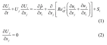
1.1 Governing equations The viscous flow around the ship is assumed incompressible and the numerical problem is described by the RANS equations coupled with the timeaveraged continuity equation in non-dimensional tensor form:

1.2 Turbulence model

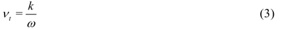
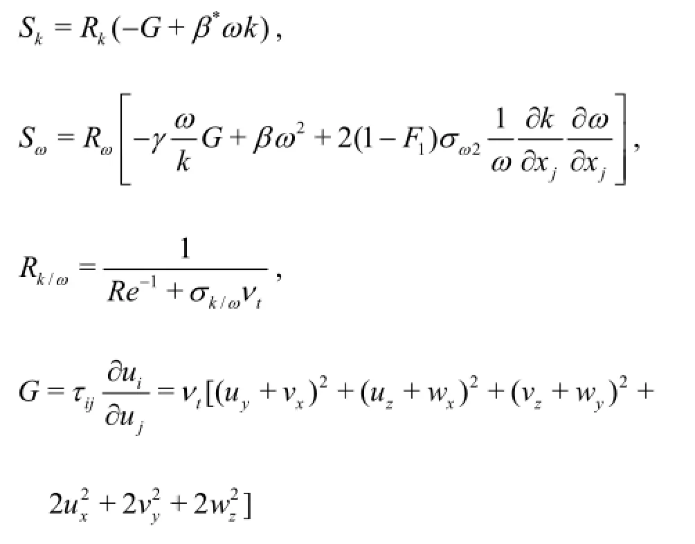
The turbulence kinetic energyis computed using a blendedmodel［25］. And in this model， the eddy viscosity， the turbulence kinetic energyand the turbulence specific dissipation ratecan be computed as:

where the source terms， the effective Reynolds numbers， and the turbulence production can be described as:

1.3 Free surface

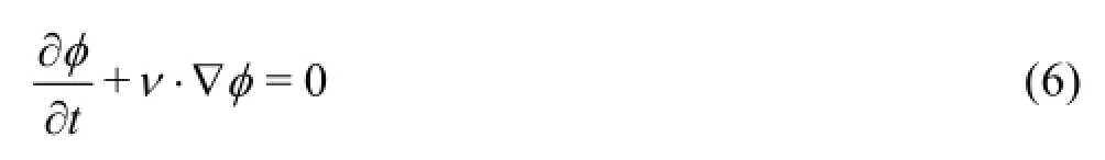
The location of the transient free surface is captured using the level set function， whose value is related to the distance to the interface. And the value ofis arbitrarily set to positive in water and negative in air and the iso-surfacerepresents the free surface. Since the free surface is considered a material interface， it should satisfy the kinematic free surface boundary condition and can be described as:

The following boundary conditions for the velocity and the pressure should be satisfied:

To make sure that the level set function remains a distance function after the transport step， a reinitialization procedure is used in which the points close to the free surface are reinitialized geometrically， while the transport equation is solved for all other points.

1.4 Coordinate transformation

The equations are first transformed from the physical domain in Cartesiancoordinates into the computational domain in non-orthogonal curvilinear coordinates. For example， the level set equation is written as

1.5 Discretization scheme

The continuity equation is discretized by using the FDM. Convective terms are discretized using a second order upwind scheme in RANS computations，and diffusion terms are discretized with a second-order central scheme.

For the temporal discretization of all equations a second-order backward scheme is used

2. Simulation design

The problem under study is a tanker model KVLCC2M with the length， moving obliquely in various water depths and drift angles incalm water at a low speed， with a Froude number of 0.142 and a model scale Reynolds number of 3.945×106. The KVLCC2M is used as a standard model for the CFDWS2005. The geometry and the principal dimensions of the model are shown in Fig.1 and Table 1， respectively.

Fig.1 Geometry of the KVLCC2M hull

Table 1 Principal dimensions of the KVLCC2M model

All studies of the present work are conducted on a computer cluster that consists of 16 Intel Xeon E5520 （2.27 GHz） processors， with 8 cores and 24 GB RAM per processor. Each computation is performed using 16 cores and takes about 54 h of the wall clock time.

Fig.2 Computational domain and boundary conditions

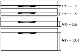
Fig.3 Four different water depths

2.1 Computational setup and boundary conditions

The computational domain covers the whole ship in view of the asymmetry of the flow field. A righthanded Cartesian coordinate system is fixed on the KVLCC2M model. The direction of theaxis is chosen along the inflow， theaxis is in the vertical direction and points upward， and the undisturbed free surface is taken as the plane. The origin of the coordinates is located at the intersection of the design water-plane， the mid-ship section and the ship center plane. A schematic diagram indicating the coordinate system and the computational domain is given in Fig.2. The boundary conditions simulate the conditions in the NMRI towing tank for later comparison of the numerical results with the experimental data. The computational domain consists of eight boundaries: the inlet plane， locatedin front of the bow， the outlet plane， locatedbehind the hulls， two ship hull surfaces， the far field， two side walls representing the shallow towing tank and the seabed wall. The total length of the computational domain isand the breadth of the computational domain is. The drift angleand the water depth vary with cases. Different drift angles， varying fromtowith an interval ofand four water depths are considered as shown in Fig.3.

Fig.4 Grid distributions in zero-drift angle case in deep water

Fig.5 Boundary layer curvilinear grid of the KVLCC2M model

2.2 Grid generation

In all cases， the structured grids are used and the overset gird technique is utilized to keep the orthogonality of the grid under the consideration of keeping a good computational accuracy of all cases. A sketch of the grid distribution of the deep water case is shown in Fig.4 and Fig.5， where the grids are coarsened forclarity. The grid consists of a background orthogonal grid， which mimics the towing tank， a refinement orthogonal grid， which covers the flow field around the hull， and a boundary layer curvilinear grid which conforms to the ship geometry where two clusters of grid points are concentrated around the bow and stern regions. The boundary layer grid is generated with a grid spacing at the hull satisfying the conditionsince no wall function is employed in the study.

The refinement grid extends within， while the background grid extends within. All the grids are refined in the vertical direction inwhere the free surface is expected.

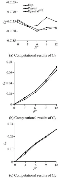
Fig.6 Hydrodynamic forces as a function of drift angle

3. Results of five benchmark test cases

First， the drift motion in deep water is computed and the predicted hydrodynamic forces， the surface pressure distribution， and the wake field are compared with the corresponding experiment data［16］to verify the current numerical methods.

3.1 Hydrodynamic forces

The hydrodynamic forces considered in this paper are， which represent thedirection force coefficient， thedirection force coefficient and the moment coefficient around theaxis， respectively. The hydrodynamic force coefficients and moment coefficient are defined as:

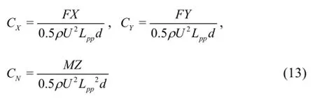
Figure 6 presents the comparison of the computed results and the experimental data for the hydrodynamic forces as a function of the drift angle. The predicted force coefficientagrees well with the measured data and with a consistent oscillation compared with the experimental data. Furthermore，changes slightly against the drift angle-increases by about only 2% fromto. The predicted force coefficientalso agrees well with the measured data and with a monotonous and rapid increase against the drift angle-increases by 475%， about 240 times the rate of， fromto. Similar tendency is also observed in the predicated results of

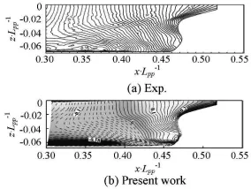
Fig.7 Surface pressure distributions at（contour line interval）

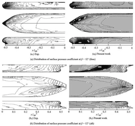
Fig.8 Distribution of surface pressure coefficients at（contour line interval）

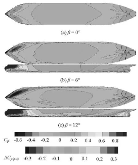
Fig.9 Pressures （top view and port side view） against drift angle in deep water

3.2 Surface pressure distribution

Comparisons of the surface pressure distribution between computed and measured results at the drift anglesandare shown in Figs.7， 8， where the pressure distributions are represented by a nondimensionalized variable， which is defined as

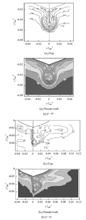
Fig.10 Axial velocity contours in WAKE 1 plane in deep water against drift angle

3.3 Wake field

In the experiment， measurements are taken at the drift anglesThe measurement plane cuts throughat the centerline of the hull. The coordinatecan be written as

The axial velocity contours（u/U） at the WAKE 1 planeagainst the drift angle in deep water are shown in Fig.10. Reasonable consistence between the computational and the experimental data can be noted. The sizes and shapes of the velocity/ wake contours of the two results are similar. Fromto， an asymmetric flow is developed as a result of the increasing drift angle， and the bilge vortex is getting stronger towards the starboard side together with an increasing wake field there.

Table 3 Predicted hydrodynamic force coefficient

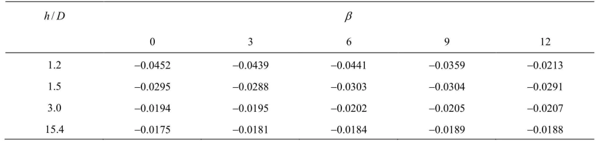
Table 3 Predicted hydrodynamic force coefficient

Table 4 Predicted hydrodynamic force coefficient

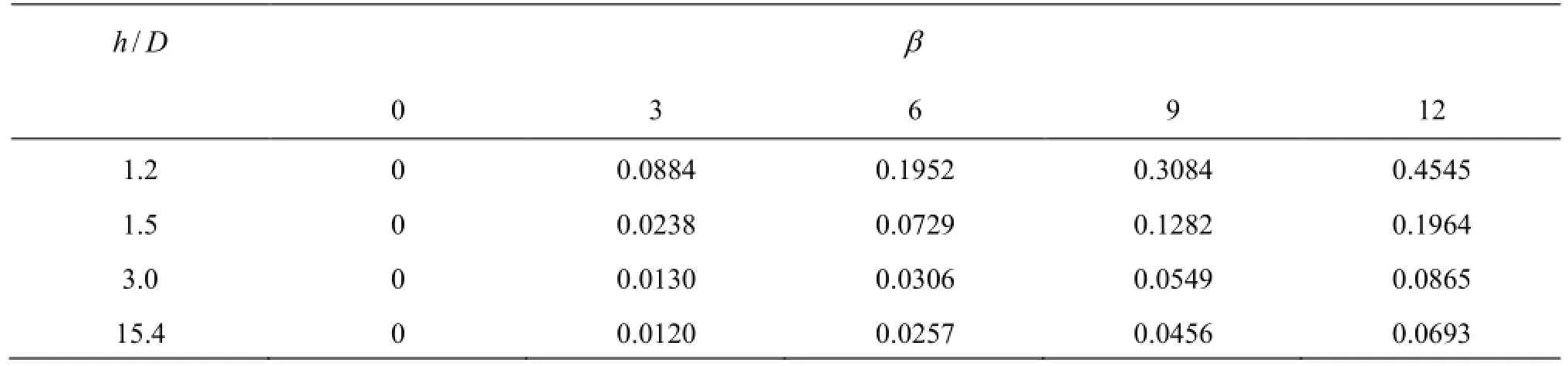
Table 4 Predicted hydrodynamic force coefficient

/ hD β 0 　3 　6 　9 　12 1.2 　0 　0.0884 　0.1952 　0.3084 　0.4545 1.5 　0 　0.0238 　0.0729 　0.1282 　0.1964 3.0 　0 　0.0130 　0.0306 　0.0549 　0.0865 15.4 　0 　0.0120 　0.0257 　0.0456 　0.0693

Table 5 Predicted hydrodynamic force coefficient

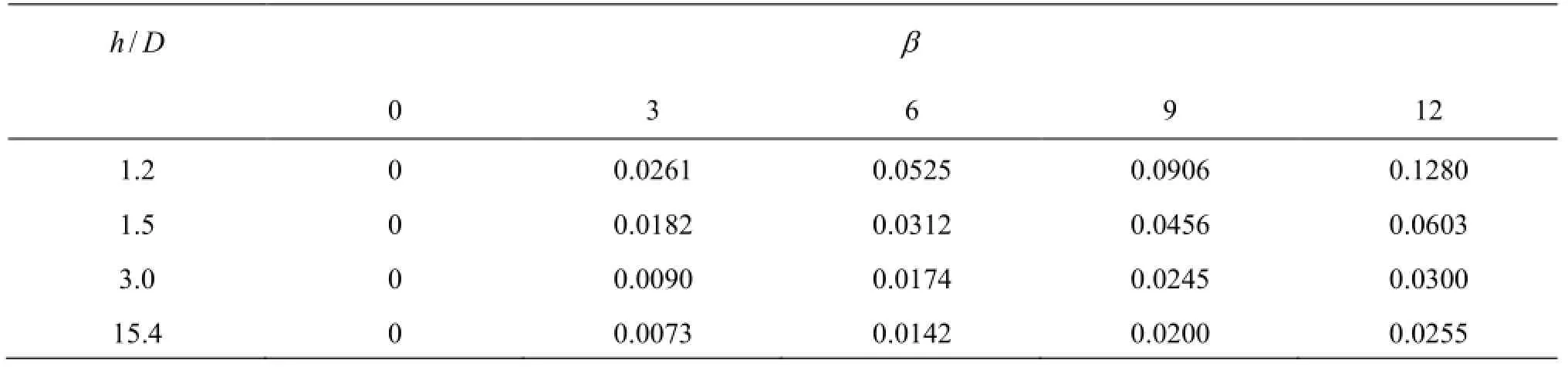
Table 5 Predicted hydrodynamic force coefficient

/ hD β 0 　3 　6 　9 　12 1.2 　0 　0.0261 　0.0525 　0.0906 　0.1280 1.5 　0 　0.0182 　0.0312 　0.0456 　0.0603 3.0 　0 　0.0090 　0.0174 　0.0245 　0.0300 15.4 　0 　0.0073 　0.0142 　0.0200 　0.0255

According to the results， the currently used numerical methods are suitable for studying the viscous flow around the hull in deep water. This method is then adopted to study the viscous flow around the hull in shallow water， which will be presented in the next section.

4. Systematic computations

In a real situation， especially， when ships are moving in ports， the water is relatively shallow. A ship’s behavior， especially， the manoeuvability， depends on the water depth to a great extent. Therefore， the viscous flow around the hull drifting in shallow water is worth studying from a general perspective.

Distinguished cases are specified （PIANC， 1992）as:

As stated in the final report of the 23rd ITTC Maneuvering Committee （23rd ITTC， 2005）， the effect of the water depth can be noticed in medium deep water， is very significant in shallow water， and dominates the ship’s behavior in very shallow water. In order to have a more clear insight into the ship maneuvering in different water depths， systematic computations are carried out. Table 2 gives the details of the test conditions for this systematic study.

4.1 Hydrodynamic forces

The predicted hydrodynamic force coefficientswith respect to various water depths and drift angles are presented in Tables 3-5， respectively. Figure 11 shows the predicted hydrodynamic force coefficientsagainst the drift angles in the shallow water case. Compared with Fig.6， Fig.11 shows rapid changes ofespecially in cases ofand. The predicted force coefficientin shallow water increasesmonotonically against the drift angle， about four times increase fromto. The same tendency can be found for the predicted force coefficient. The results indicate that the effect of water depth is significant， as is consistent to the common sense of naval architects.

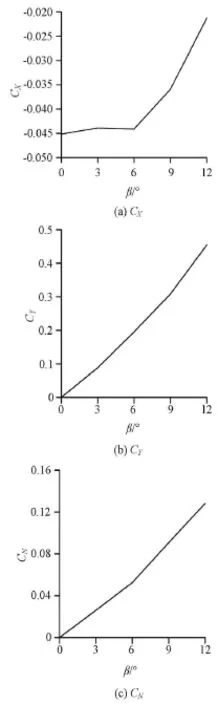
Fig.11 Results in shallow wateragainst drift angle

Results of the predicted hydrodynamic force coefficientsagainst various water depths are shown in Fig.12. The results also indicate the significant effect of water depth. The predicted hydrodynamic forces change a great deal when the water depth changes fromtoespecially， for the lateral force coefficientand the moment coefficient， which increase about six times and three times， respectively. However， when the water depth is greater than， the hydrodynamic forces change very slightly. The lateral force coefficientonly changes 1.18 times， when the water depth changes fromto15.4. So， the computated results satisfactorily confirm the normally accepted view that the shallow water effects is not so serious until the water depth is below3.0.

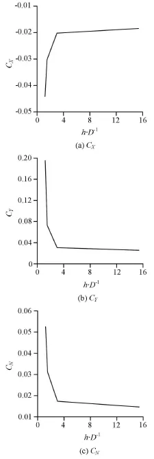
Fig.12 Results atagainst water depth （1.2， 1.5，3.0， 15.4）

4.2 Surface pressure distribution

The predicted pressure distributions on the ship hull （as the main contributor to the lateral force coefficientand the yaw moment coefficientare shown for better understanding the computed forces and moments. In Figs.13， 14， the pressure distributions （， nondimensionalized by0.5ρU2） on the hull surface together with the pressure difference between the port and the starboard sidesare depicted under different conditions， where the solid lines stand for positive values and dotted lines represent negative values. The pressure difference in the case ofis not given， as the flow is symmetric.

Fig.13 Pressure （bottom view） and pressure difference （at port side） distributions against drift angle in shallow water

Compared with Fig.9， Fig.13 shows the pressure reduction in shallow water for the same variation of the drift angle is considerably more significant， as indicated by the two large low pressure regions on the hull bottom. The results also indicate that the low pressure peaks are not only because of the hull surface curvature but also due to the influence of the small under keel clearance. The two low pressure regions grow in size and decrease in value with the increase of the drift angle.

Fig.14 Pressure （bottom view） and pressure difference （at port side） distributions against water depth

Fig.15 Axial velocity contours on wake 1 plane against drift angle in shallow water

Similarly， with a larger positive pressure difference on the fore-body and the negative difference on the aft-body， a positive lateral force coefficientand yaw moment coefficienttoward the starboard side are then generated. Compared with Fig.9，Fig.13 shows a larger pressure difference on the hull surface in shallow water， which may explain the produc tion o f the l arg er for ces and m oments sho wn in Fig.16thanthoseindeepwaterasshowninFig.6.With a greater depth at， the shallow water effects are gradually alleviated， as shown in Fig.14（c）and Fig.14（d）. Comparing Fig.14（c） and Fig.14（d），rather similar pressure results atandcan be noticed， which demonstrates again that the shallow water effect is very small for， which further supports the results and discussions with respect to Fig.12.

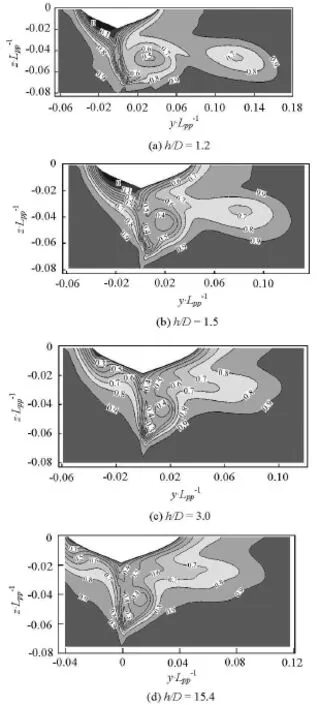
Fig.16 Axial velocity contours on wake 1 plane against water depth

4.3 Wake field

Details of the computed flow field are shown to see the shallow water effects. First， the axial velocity contoursat wake 1 planunder shallow water conditions against the drift angle are shown in Fig.15， while the contours with varying water depths at the drift angleare shown in Fig.16.

Under the shallow water condition， as shown in Fig.15（a）， the flow remains symmetric whenHowever， as a result of the blockage of the seabed， the axial velocity outside the boundary layer increases. Moreover， a pronounced flow separation appears. In the non-zero drift angle case， with the caseas an example， the flow becomes asymmetric and the separation area is reduced to some extent， which moves toward the starboard side and partly upwards towards the transom. Comparing the results in the case ofin deep water （Fig.10） and in shallow water（Fig.15）， a larger bilge vortex is detached from the hull on the starboard side and a second vortex is developed near the keel in shallow water. Moreover， a separation area is produced on the port side close to the hull. And in the case of， though the separated area appears to have become smaller， the second weaker vortex arises.

Fig.17 Wave pattern against drift angle in shallow water（h/

Figure 16 depicts the influence of water depth aton the axial velocity contours at1.2， 1.5， 3.0， 15.4. A clear tendency of the increasing wake field and vortex strength with a decreasing water depth can be noted. Furthermore， comparing the results of the axial velocity contours for（Fig.16（c）） and（Fig.16（d））， the difference is undiscernible， indicating that the shallow watereffect is almost negligible for， which further supports the results and discussions with respect to Fig.12 and Fig.14.

4.4 Wave pattern

To provide a further insight of the effects of shallow water and drift angle， the computed wave pattern is shown. The wave pattern in shallow water cases against the drift angle is shown in Fig.17， while the wave patterns with varying water depths at the drift angleare shown in Fig.18.

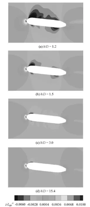
Fig.18 Wave pattern against water depth

Under the shallow water condition， as shown in Fig.17（a）， the flow remains symmetric whenIn the non-zero drift angle case， as shown in Fig.17（b），the flow becomes asymmetric and the difference of the water level around the port and the starboard side is shown. With the increase of the drift angle， the water level on the two sides of the ship becomes asymmetric and the water level difference around the two sides appears to be more pronounced. The water level around the starboard-side is lower than that on the port-side around the bow， which produces a positive pressure towards the starboard. Moreover， the starboard-side water level is higher than that on the portside around the stern， which produces a negative surface pressure towards the port. However， the size and the value of the water level difference around the stern are very small so that the contribution to the surface pressure is accordingly small. As a result， a positive surface pressure pointing to the starboard-side is finally produced. With a larger drift angle， the water level differences on the fore-body and the aft-body both increase. However， the value of the water level difference on the fore-body is larger and it increases faster，so the water level difference on the fore-body dominates and it produces an increased positive surface pressure. Figure 18 shows the influence of the water depth aton the wave pattern with1.2， 1.5， 3.0， 15.4. A clear tendency of increasing water level difference with decreasing water depth is noticed. On the other hand， comparing the results of the wave pattern for（Fig.18（c）） and（Fig.18（d））， the water level difference around the two sides of the ship is almost undiscernible， which indicates that the shallow water effect is almost negligible for

5. Conclusions

Unsteady RANS simulations of the drift motion of a KVLCC2M model in both deep and shallow waters are presented. The hydrodynamic forces and moments， the surface pressure distribution and the wake field are obtained. In general， the computed results， which give a clear insight into the forces and moments acting on the ship as a function of drift angle or water depth， agree well with experimental data with respect to the tendencies of the forces and moments. Major findings are:

（1） The numerical errors are less than 3% for all three variables in all deep water cases， which implies that the present method is a promising tool for the prediction of the hydrodynamic forces acting on a ship moving obliquely.

（2） In the shallow water cases， the flow field analyses show the shallow water effects， as well as the influence of the oblique flow on the forces and moments， which supports the normally accepted opinion that only when the water depthis below 3.0， theshallow water effects can be noticed.

（3） In the large drift angle cases， the orthogonality and the quality of the grid are provided by the overset technique， which is not only easy for the structure grid generation and the local grid refinement， but also without the grid distortion in large drift angle cases. The practicability of the overset grid technique for simulating ship motions in confined waters is shown by the results.

Acknowledgements

This work was supported by the Chang Jiang Scholars Program （Grant No. T2014099）， the Program for Professor of Special Appointment （Eastern Scholar）at Shanghai Institutions of Higher Learning （Grant No. 2013022） and the Innovative Special Project of Numerical Tank of Ministry of Industry and Information Technology of China （Grant No. 2016-23/09）， to which the authors are most grateful.

References

［1］ TOXOPEUS S. L.， SIMONSEN C. D. and GUILMINEAU E. Investigation of water depth and basin wall effects on KVLCC2 in manoeuvring motion using viscous-flow calculations［J］. Journal of Marine Science and Technology， 2013， 18（4）: 471-496.

［2］ KIM B.， SHIN Y. S. A NURBS panel method for threedimensional radiation and diffraction problems［J］. Journal of Ship Research， 2003， 47（2）: 117-186.

［3］ MAIMUN A.， PRIYANTO A. and SIAN A. Y. et al. A mathematical model on manoeuvrability of a LNG tanker in vicinity of bank in restricted water［J］. Safety Science，2013， 53（2）: 34-44.

［4］ ZOU L.， LARSSON L. Numerical predictions of ship-toship interaction in shallow water［J］. Ocean Engineering，2013， 72: 386-402.

［5］ VANTORRE M.， DELEFORTRIE G. Behaviour of ships approaching and leaving locks: Open model test data for validation purposes［C］. 3rd International Conference on Ship Manoeuvring in Shallow and Confined Water: with Non-Exclusive Focus on Ship Behaviour in Locks. Ghent， Belgium， 2013， 1-16.

［6］ SUTULO S.， RODRIGUES J. M. and SOARES C. G. Hydrodynamic characteristics of ship sections in shallow water with complex bottom geometry［J］. Ocean Engineering， 2010， 37（10）: 947-958.

［7］ STERN F.， WANG Z. and YANG J. et al. et al. Recent progress in CFD for naval architecture and ocean engineering［J］. Journal of Hydrodynamics， 2015， 27（1）: 1-23.

［8］ SHEN Z. R.， WAN D. C. RANS Computations of added resistance and motions of ship in head waves［J］. International Journal of Offshore and Polar Engineering， 2013，23（4）: 263-271.

［9］ CAO H. J.， WAN D. C. Development of multidirectional nonlinear numerical wave tank by naoe-FOAM-SJTU solver［J］. International Journal of Ocean System Engineering， 2014， 4（1）: 52-59.

［10］ CAO Hong-jian， WAN De-cheng. RANS-VOF solver for solitary wave run-up on a circular cylinder［J］. China Ocean Engineering， 2015， 29（2）: 183-196.

［11］ SHEN Zhi-rong， WAN De-cheng. An irregular wave generating approach based on naoe-FOAM-SJTU solver［J］，China Ocean Engineering， 2016， 30（2）: 177-192.

［12］ SIMONSEN C. D.， STERN F. Verification and validation of RANS maneuvering simulation of Esso Osaka: Effects of drift and rudder angle on forces and moments［J］. Computers and fluids， 2003， 32（10）: 1325-1356.

［13］ WANG Hua-ming， ZOU Zao-jian and TIAN Xi-min. Computation of the viscous hydrodynamic forces on a KVLCC2 model moving obliquely in shallow water［J］. Journal of Shanghai Jiaotong University （Science），2009， 14（2）: 241-244.

［14］ ZOU L. CFD predictions including verification and validation of hydrodynamic forces and moments on a ship in restricted waters［D］. Doctoral Thesis， Gothenburg，Sweden， Chalmers university of Technology， 2012.

［15］ EÇA L.， HOEKSTRA M. and TOXOPEUS S. Calculation of the flow around the KVLCC2M tanker［C］. CFD Work-shop Tokyo. Tokyo， Japan， 2005.

［16］ KUME K.， HASEGAWA J. and TSUKADA Y. et al. Measurements of hydrodynamic forces， surface pressure，and wake for obliquely towed tanker model and uncertainty analysis for CFD validation［J］. Journal of Marine Science and Technology， 2006， 11（2）: 65-75.

［17］ MENG Q. J.， WAN D. C. Numerical simulations of viscous flows around a ship while entering a lock with overset grid technique［C］. The Twenty-fifth International Ocean and Polar Engineering Conference. Kona， Hawaii Big Island， USA， 2015， 4: 989-996.

［18］ ROGERS S. E.， SUHS N. E. and DIETZ W. E. PEGASUS 5: An automated preprocessor for overset-grid computational fluid dynamics［J］. AIAA Journal， 2003， 41（6）: 1037-1045.

［19］ TAHARA Y.， WILSON R. V. and CARRICA P. M. et al. RANS simulation of a container ship using a single-phase level-set method with overset grids and the prognosis for extension to a self-propulsion simulator［J］. Journal of Marine Science and Technology， 2006， 11（4）: 209-228.

［20］ CARRICA P. M.， WILSON R. V. and NOACK R. W. et al. Ship motions using single-phase level set with dynamic overset grids［J］. Computers and Fluids， 2007， 36（9）: 1415-1433.

［21］ CHAN W. M. Overset grid technology development at NASA Ames Research Center［J］. Computers and Fluids，2009， 38（3）: 496-503.

［22］ CARRICA P. M.， ISMAIL F. and HYMAN M. et al. Turn and zigzag maneuvers of a surface combatant using a URANS approach with dynamic overset grids［J］. Journal of Marine Science and Technology， 2013， 18（2）: 166-181.

［23］ SHEN Z. R.， WAN D. C. and CARRICA P. M. Dynamic overset grids in OpenFOAM with application to KCS selfpropulsion and maneuvering［J］. Ocean Engineering，2015， 108: 287-306.

［24］ XING T.， BHUSHAN S. and STERN F. Vortical and turbulent structures for KVLCC2 at drift angle 0， 12， and 30 degrees［J］. Ocean Engineering， 2012， 55: 23-43.

［25］ MENTER F. R. Two-equation eddy-viscosity turbulence models for engineering applications［J］. AIAA Journal，1994， 32（8）: 1598-1605.

［26］ OSHER S.， SETHIAN J. A. Fronts propagating with curvature-dependent speed: algorithms based on Hamilton-Jacobi formulations［J］. Journal of computational physics， 1988， 79（1）: 12-49.

June 24， 2015， Revised November 25， 2015）

* Project supported by the National Natural Science Foundation of China （Grant Nos. 51379125， 51490675， 11432009，51579145 and 11272120）.

Biography: Qing-jie MENG （1986-）， Male， Ph. D.

De-cheng WAN，

E-mail: dcwan@sjtu.edu.cn