Oscillating-grid turbulence at large strokes: Revisiting the equation of Hopfinger and Toly*

Wan Hanna Melini WAN MOHTAR

Department of Civil and Structural Engineering， Faculty Engineering and Built Environment， Universiti Kebangsaan Malaysia， Bandar BaruBangi 43600， Selangor， Malaysia， E-mail: hanna.mohtar@gmail.com



Oscillating-grid turbulence at large strokes: Revisiting the equation of Hopfinger and Toly*

Wan Hanna Melini WAN MOHTAR

Department of Civil and Structural Engineering， Faculty Engineering and Built Environment， Universiti Kebangsaan Malaysia， Bandar BaruBangi 43600， Selangor， Malaysia， E-mail: hanna.mohtar@gmail.com

A quasi-isotropic， quasi-homogeneous turbulence generated by an oscillating-grid， spatially decays according to power law of， whereis the root mean square （rms） horizontal velocity，Z is the vertical distance from the grid andHowever， the findings of Nokes and Yi indicate that as the stroke of oscillation increases， the power lawan d does not follow the established decay law equation of Hopfinger. This paper investigates the characteristics of the turbulence that are generated using larger strokes1.6 and 2 and compares with that obtained using a， which is the stroke used when the equation was developed. Measurements of the grid-generated turbulence in a water tank were taken using particle image velocimetry （PIV）. The results showed that the homogeneity occurred at distance beyond 2.5 mesh spacings away from the grid midplane， independent of the stroke and the frequency of oscillation. Within this region， the turbulent kinetic energy distribution was quasi-homogeneous， and the secondary mean flow is negligible. The statistical characteristics of the measured turbulence confirmed that althoughdecreases as stroke increases， the grid-turbulence generated at1.6 and 2 obeys the universal decay law.

oscillating-grid turbulence， large strokes， decay power law

Introduction

The effect of turbulence as an environmental variable in geophysical phenomena is important and has drawn ever increasing attention recently. Turbulence plays a significant role in the critical motion of sediment， particles suspension and contaminant dispersion， to name a few. As the characteristics of the turbulence are random in time and space， measuring the velocity representing the turbulence is difficult and complex. Nevertheless， the turbulent flow can be represented rather simply by employing an oscillatinggrid in a contained water tank［1-3］. In a laboratory frame， the flow at distances further away from the grid is statistically stationary and the turbulence statistics of the transversal velocity componentsonly vary in the direction perpendicular to the grid planeUtilising this frame of reference， the grid turbulence can be modelled as statistically homogeneous and isotropic flow， which allow relatively complete statistical information to be provided by fewer measurements than is required for the classical shear flows. Various geophysical phenomena have been studied using this kind of turbulent flow， including the particle-turbulence interaction［4］， the incipient sediment motion［5-7］， the turbulence evolution near a wall or a free surface［8］， the desorption of contaminants from sediment［9］， the aggregation of particle dynamics［10］，the air-water interface［11］and aquatic vegetation［12］.

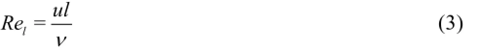
The dynamical equation governing these turbulence components can be derived by applying the Reynolds decomposition［2］. Incorporating the grid geometry’s external parameters， including the oscillation frequencyand the oscillation stroke， the root mean square （rms） horizontal velocity component（and by proposing a similar derivation for the rms vertical velocity component（due to isotropy）），Hopfinger［1］represented the turbulence characteristics as

Equation （1） is developed based on the fact that the integral length scale is linearly increased with the distance from the grid mid-position as

Equation （1） suggests that increasing the stroke and the frequency of the oscillation increasesand subsequently increases. Previous findings have shown that the upper limit of the frequency is between 6 Hz to 7 Hz， where values above this upper limit will generate a significant secondary flow［13-15］. Note that by using stroke， the maximum achievable（with frequency of 6 Hz） before the secondary circulation becomes significant is only approximately 300. Thus， a larger stroke must be used to increase the flow strength. Although this idea has been suggested，there are quite a few studies that have used an， while very limited research has focused on the validity of Eq.（1） using larger strokes. Most of the previous studies used strokes comparable to those used by Hopfinger［1］（i.e.，）， whose proposed model has been generally accepted as correct［7，9］. The findings of Nokes［16］and Yi［17］who used rangebetween 0.15-0.98 and， respectively， however found out that the power lawis dependent on the stroke， wheredecreases （i.e.，） with increases in stroke of oscillation. This implies that the turbulence generated decays much slower and the presence of the secondary circulation is significant. Although their work used similar range strokes of， their findings were not in agreement with Hopfinger［1］. They suggest that a non zero-mean turbulence is generated using larger stroke and， the representation of the quasi-isotropic， homogeneous turbulence using Eq.（1） is rendered invalid.

These contradictory findings motivate this paper to experimentally investigate the characteristics of the generated grid turbulence by systematically increase the strokes. The main body of this paper will focus on the response of the grid-generated turbulence using larger strokes， in particular the onset of the homogeneous region， the linearity of the integral length scale and the determination of the decay power laws are discussed in detail.

Fig.1 Schematic drawings of （a） the front view of experiment apparatus and （b） the plan view of the grid. Symbolsanddenote the angle of the tilted tank and the distance from the virtual origin， respectively. Note thatthroughout the experiments. In （b） A-A， which is aligned with the central bar at the centre of the grid denotes where the light sheet is illuminated

1. Experimental apparatus and procedure

The experiments were performed in an acrylic tank， with cross-sectional dimensions of 0.00354× 0.00354 m2and a height of 0.5 m. The tank is fixed within a rigid inner steel frame and filled with water to a depth of 0.4 m. The oscillating-grid mechanism，consists of a linear bearing was positioned vertically through the central axis of the tank and connected to a rotating spindle. A motor is used to rotate the spindle and thus continuously oscillate the grid. The plan view of the square， uniform grid shown in Fig.1（a） made from 7×7 array of aluminum bars and length of 0.35 m. The uniform mesh sizeis 0.05 m and gives the grid a solidity of 0.36. The end condition of the grid is designed to ensure that the wall acted as a plane of reflection-symmetry， whichhas been shown to lessen the Reynolds-stress gradients within the fluid， thereby inhibiting the presence of undesirable secondary circulations （see De Silva［13］for a detailed discussion）. The opening between the wall and the grid is approximately 0.002 m， which is very small to cause any significant secondary circulation［18］.

Table 1 Summary of the experimental setup

The velocity measurements were obtained using two-dimensional planar particle image velocimetry（PIV）， applied in the verticalplane through the centre of the tank. The reflective， neutrally buoyant tracer particles were illuminated using a narrow， vertical light sheet （with a thickness of 0.002 m） that was directed through the mid-plane of the tank （Section A-A as shown in Fig.1（b））. The motion of the tracer particles was recorded using a high-speed DantecNanoSenseMkIII digital camera（with 1 280×1 024 pixel resolution） and the frame rate is set at 200 Hz. The camera was positioned to have a vertical light-sheet through the mid plane of the tank. In each case， the velocity profiles were calculated from pairs of images with a cross-correlation algorithm using a standard PIV software. The interrogation area was set at 20×20 pixels （equivalent to 0.00019× 0.00019 m）， with a 50% overlap between the analysis spots. For each experimental setup， the velocity fields were acquired for a period of 120 s， which provided the spatial and the temporal data of the horizontal and vertical velocity components in the bulk fluid. The measurement of velocity using PIV allows a planar flow distribution to be obtained， from the bottom of the grid （i.e.，） to the tank base， giving a physical region of approximately 0.0025×0.003 m2. Note that however， for each stroke， to include both bottom of the grid and the tank base in the visualisation， the camera was readjusted and thus， gives a variation of the planar flow area.

2. Results and discussion

2.1 Mean flow

It is relatively difficult to completely eliminate the secondary flow in the OGT system and such flow should be recognized as an intrinsic feature in the oscillating-grid turbulence［19］. Even so， in this study，care was taken to minimize the secondary flow in the oscillating-grid tank. As mentioned previously， the grid employed had a solidity of 0.36， comprised of square-bars and had grid end conditions such that the wall behaved as a plane of symmetry. The maximum frequencythat was used in this study was 6 Hz， which is below the recommended limits of 7 Hz and 8 Hz［15］.

In an attempt to qualitatively ascertain that the mean flow was weak in the grid tank， the time-averaged mean velocity fields measurements were observed. The PIV results provided whole-field visualisations of the bulk flow structure with an area of. Representatives of twodimensional illustration of the mean velocity fields and the distribution of turbulent kinetic energy that were produced in theplane are shown in Fig.2 for turbulent flow with0.8 and 1.6. Note that due to the camera readjustment， thefor Figs.2（a） and 2（b） were 5 and 6， respectively. This however is insignificant asis fixed and the depth includes the bottom of the grid and the tank base. The turbulent kinetic energy （per unit mass）was defined aswhere the assumption of transversal isotropyhas been used.

Fig.2 The mean velocity fieldsand the turbulent kinetic energy distributionin theplane， The down arrow （↓） on the top right indicates the maximum mean velocity value and the colour bar represents the strength of the turbulent kinetic energy

Because of the no-slip condition at the surface of the grid elements， each bar generated vorticity due to the viscous forces at the edge of the grid， producing alternating negative and positive vorticities. The high vorticity distribution near the grid is due to the presence of shear stresses， which are the result of the wake and the jet that were produced from the movement of oscillating-grid. The interaction of the jet and the wakes creates a layer of intense turbulent motion and a high intensity turbulent kinetic energy. The turbulent layer is thickened via the entrainment of the irrotational surrounding fluid， giving rise to large-scale energetic motions， particularly around1 to 2. Consistent coupled negative and positive rotations （for example atin Fig.2（a）） near grid are scaled at approximately. The mean flow mapping at near grid shows the symmetrical characteristics about the tank plane.

Both figures show persistent jet structures in the middle of the tank and travel up to. At a distance offrom the grid， the intense interaction between the jets and the wakes breaks down into turbulence. After， there is a reduced spatial variability and theis quasi-homogeneously distributed across the x direction for a given depth further away from the grid. Obviously， a higher（as shown in Fig.2（b）） produced higher turbulent kinetic energy at near grid and took longer distance to reach homogeneity. Nevertheless， at， there is an insignificant shear stress and negligible large scale motions in the bulk flow， indicating no significant secondary circulations within the tank.

Results show that the mean flow is an inherent feature in an oscillating-grid tank particularly at near grid， in agreement with McKenna［19］. However， the ratio of the rms velocity to the mean velocityis examined to gauge the level ofthe turbulence intensity produced. For the range ofdiscussed in this article， the horizontal turbulent intensityranged from 2-10， whereas the vertical turbulent intensityranges from 1-6. This indicates that the turbulence is the dominant component than the mean flow within the tank. Smaller turbulence intensity values were observed for the vertical components， in whichis relatively higher due to the vertical direction of the grid oscillation.

Fig.3 Evolution of the degree of isotropyfor. Errorbars show the variability observed in the data

2.2 Onset of the quasi-isotropic homogeneous turbulence

Although Fig.2 showed that negligible secondary mean circulations can be found from， the onset of the quasi-isotropic homogeneous turbulence region was determined by plotting the isotropy， from grid bottom i.e.，toto eliminate the inhomogeneity effects due to the presence of the （solid） tank base. Secondary circulations were observed when the turbulence interacted with the tank base， resulting in local inhomogeneity and anisotropy［20］. Figure 3 shows the evolution of the degree of isotropy， as a function of the distance for0.8， 1.6 and 2 with theranging from 67 to 607. Data consistently shows that throughout the depth， the componenthas a larger value than，? particularly at a close proximity to the grid. Althoughwas not ideally 1， the isotropy value remained constant （at least within the experimental error）， at distances. The errors associated were determined as the standard deviation from the measurement of spatially averaged value ofand， at each. Isotropy increases with larger strokes， withvalues of 1.1， 1.3 and 1.5 for0.8， 1.6 and 2， respectively， where these values falls within the acceptable range with previous studies［14］. As such， it can be considered that the “quasi-isotropic homogeneous turbulence” region starts at， regardless of the stroke and the frequency of the oscillation. Even so， it should be stressed here， that due tothe grid turbulence generated is not an isotropic flow.

2.3 Integral length scale

To derive Eq.（1）， the integral length scale of the turbulence needs to be linearly dependent onwithin the “quasi-isotropic homogeneous turbulence” region. The longitudinal integral length scalewas obtained using the same approach adopted by Thompson［2］， as the area under the auto-correlation function of the horizontal velocity component.

Fig.4 The integral length scalesplotted linearly against the distance Sediment incipience in turbulence generated ina square tank by a vertically oscillating-grid， where data are represented with the turbulence that was generated. The errors associated with the measurement ofare also shown， where the smaller error bar represents minimum error and larger error bar shows the maximum error range

The computed integral length scalelfor0.8， 1.6 to 2 are plotted as a function of depth， here shown in Fig.4. Note that the data is plotted according to each stroke for better illustration. Using a line fit from the method of least squares， a linear relationshipwas obtained， and values offor each stroke were computed， shown here in Table 2. Althoughis found to increase with， all of the values are well within the range of 0.1-0.3 that was reported in previous studies［1］. As anwas used here， the scale should only proportional to［1］. However， for a given mesh sizedescribed in the experiments （i.e.， fixed at 0.05 m）， the coefficientwas found to increase asincreases. In all cases， Eq.（1） is validated and the least squares fit for all data gives

Table 2 Summary of the coefficients â for each stroke used

The estimation of the maximum and the minimum error associated with the measured values ofare also shown in Fig.4. The error is calculated as the standard deviation from time averagingover120 s. The variation of the error is somewhat pessimistic and is likely due to the arbitrary calculation of the integral length scale itself. The minimum error that is associated with themeasurements occurs within the specified homogeneous region that is closer to the grid， whereas the maximum error occurs at a larger. As the turbulence spatially decays， the smallest eddies decay the fastest due to their small turn over time compared to the larger scale eddies. Thus， large，slowly rotating eddies dominate the turbulence region that is further away from the grid. That is when calculatingat this distance， the correlation of horizontal velocity of large eddies across theaxis is less autocorrelated， resulting in a higher error.

2.4 The spatial decay of the quasi-isotropic homogeneous turbulence

The isotropy plot shows that the quasi-isotropic homogeneous region starts at approximately2.5M away from the grid. As mentioned previously， Eq.（1）is only applicable within the homogeneous turbulence region. The inhomogeneity of the turbulence near the grid， if included in the region that is used to calculate the empirical coefficients（i.e.，andwill have a significant impact on the determination of these coefficients and their values may vary by up to 20%［18］. From Eq.（1）， the spatially averaged rms horizontal and vertical velocity components with distancebelow the grid mid position are presented as

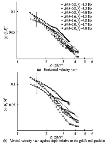
Fig.5 Measurements of the （spatially averaged） rms. against depth relative to the grid’s mid-position. Hereandhave been dimensionless usingand， respectively. The straight line shows the least-squares fit for all of the data. To avoid saturation， a single error bar has been included in each plot that is representative of the variability observed in all data

The assumption of quasi-isotropic turbulenceat a fixed distance， suggests that theThus， there are few studies that examine the vertical velocity empirical constants. To the best of the author’s knowledge， only two studies by De Silva［13］and Yi［17］have examinedand， where De Silva［13］only investigated thefor one stroke. Using stroke， they found thatHowever， Yi［17］who used multiple strokes in his experiments （i.e.，） discovered that the power lawvalues are dependent on the stroke， withdecreasing asincreases. The limited number of investigations that focus on， as well as the mixed results that were obtained from these studies， encouraged further analysis to assess the vertical power decay lawby plotting the data according to Eq.（5b）， here shown in Fig.5（b）.

The results are now discussed. The measured data shows that the decay exponent rms. horizontal velocity componentsis 1.22， where this value is comparable to， found by Hopfinger［1］. The difference of measuredwith Hopfinger［1］’s is about 18%， in line with the findings of George［18］. This is believed to be contributed by the varying onset homogeneous region taken when the coefficients were obtained. Hopfinger［1］considered the onset as0.7， much closer to the grid， where as here， the homogeneous region was taken from， the region whereand the effect of large scale motion from the turbulence production region near grid is minimal. At distance， as shown in Fig.2， the large scale motion is significant and will essentially have affected the coefficient values.

The vertical turbulence component however， decay much faster withbecause the vertical energy is used to transport the kinetic energy. The data also gives the empirical coefficients ofand， respectively and are found to be within the range values of Hopfinger［1］who foundand. The variations ofandare expected due to the different oscillating-grid setup for each study. With the valuesandobtained in this study， theandcomponents are underestimated by about 40% and 20%， respectively than when the empirical coefficients of Hopfinger［1］were employed.

Table 3 Summary of the coefficientsandand the decay law exponentsnuand nw

Table 3 Summary of the coefficientsandand the decay law exponentsnuand nw

/ SMunwnuCwC 0.8 　1.22 　1.43 　0.14 　0.19 1.6 　0.94 　0.99 　0.12 　0.17 2.0 　0.92 　0.93 　0.12 　0.16

Table 4 Comparison of the decay law exponentsandobtained by Nokes［16］， Yi［17］and this study

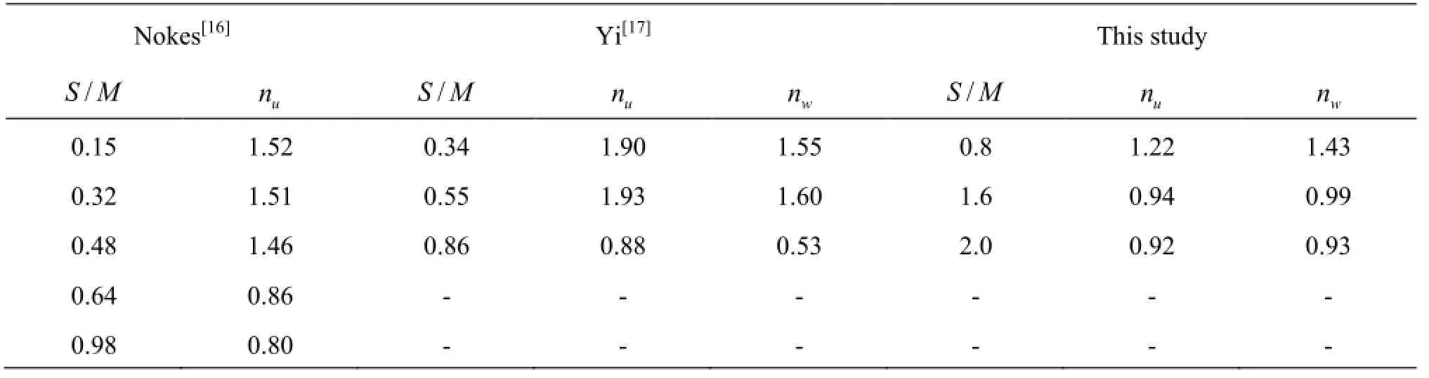
Table 4 Comparison of the decay law exponentsandobtained by Nokes［16］， Yi［17］and this study

?

What is more important is that bothandare of similar orders of magnitude.

The analysis also shows that the turbulence decays much faster withfor， in particular thecomponent with a distinguished deviation betweenandis approximately. This is due to the smaller vertical length scale， in which the large scale eddies break up into smaller scales more quickly than in larger horizontal length scales. However， with increasing strokes （i.e.， increasing the turbulent Reynolds numbers）， the differences between the constantsanddiminish， and they both approach unity. The decay of the turbulence that is produced by strokes of0.8， 1.6 and 2 show power laws of1.22， 0.94， 0.92， and1.43， 0.99， 0.93， respectively. These results indicate that the use of a larger stroke （within）， produced a quasi-isotropic homogeneous turbulence that follows the established decay law of Hopfinger［1］.

The comparison of coefficientsandwith the values obtained by Nokes［16］and Yi［17］is now discussed. Both studies which used， as shown in Table 4， evidently show a decreasing trend asincreases. However， whenis comparable to the one used by Hopfinger［1］the decay law， much lower than 1. Data of Nokes［16］shows a consistent profile for smaller strokes， where the velocity decay was closer to， in agreement with Thompson［2］. Although Yi［17］showed that thevelocity component decays according to， the measuredforhowever were essentially out of the range. Both studies are somehow interesting as they indicate that the characteristics of the grid turbulence generated atis not a quasi-isotropic homogenous turbulence. Looking at their decreasing trend， it is suggested that for， the grid turbulence do not obey the law. This paper however， able to show that even at larger strokes， the behaviour of the generated grid turbulence is accordance with the established universal decay law［1］.

3. Conclusions

The experiments reported here examined the characteristics of an oscillating-grid generated turbulence， with attention focused on larger strokes （1.6 and 2） and compared with the turbulence characteristics generated with the stroke（that is the stroke used to develop the universal decay law by Hopfinger［1］）. Previous oscillating-grid studies usedstroke and generally accepted the validity of Eq.（1）. This reliability of the equation however， wasquestioned by Nokes［16］and Yi［17］where they found that asincreases the decay lawand Eq.（1） is invalid. Here， the analysis was extended to consider larger strokesand examine the characteristics of generated turbulence in terms of mean flow，evolution of isotropy， the linearity of integral length scale and the determination of power decay laws.

The grid-generated turbulence was found with negligible mean shear flow and insignificant secondary circulations at distances further away from the grid， approximately at. Using the analysis of isotropy， it is shown that the generated turbulence is not isotropic， where the value of isotropy. However， it can be said that the “quasi-isotropic homogeneous turbulence” region， starts at， independent of stroke and frequency of the oscillation. These observations are consistent with the turbulence profile generated withstroke， identified in this study and previous research［1，19］.

The data reported here show a decrease in the empirical decay lawsandwhenin agreement with findings of Nokes［16］and Yi［17］. Although， the measured value ofatwas approximately 1， and corresponded well with the results of Hopfinger［1］. The determination ofwas notably unaccounted for in the past studies， and is usually accepted asdue to the isotropic behaviour. Here， the analysis was expanded to investigate the vertical power decay law. The measured values ofwere higher thanforandand w n reached unity at approximately 0.92 for. The higherwas expected as the grid is vertically oscillated， where the energy of the vertical component is used to transport the turbulent kinetic energy down to the tank bottom， leading to a faster decay of the vertical velocity components.

Acknowledgements

The author gratefully acknowledges Damien Goy and Mike Langford for the technical support provided and Universiti Kebangsaan Malaysia for the financial support during the author’s postgraduate studies.

References

［1］ HOPFINGER E. J.， TOLY J. A. Spatially decaying turbulence and its relation to mixing across density interfaces［J］. Journal of Fluid Mechanics， 1976， 78: 155-175.

［2］ THOMPSON S. M.， TURNER J. S. Mixing across an interface due to turbulence generated by an oscillatinggrid［J］. Journal of Fluid Mechanics， 1974， 67: 349-368.

［3］ PUJOL D.， COLOMER J. and SERRA T. et al. Effect of submerged aquatic vegetation on turbulence induced by an oscillating-grid［J］. Continental Shelf Research， 2010，30（9）: 1019-1029.

［4］ POELMA C. Particle-fluid interactions in grid-generated turbulence［J］. Journal of Fluid Mechanics， 2007， 589: 315-351.

［5］ WAN MOHTAR W. H. M.， MUNRO R. J. Threshold criteria for incipient sedimentmotion on an inclined bedform in the presence of oscillating-grid turbulence［J］. Physics of fluids， 2013， 25（1）: 015103.

［6］ LIU C.， HUHE A. and TAO L. Sediment incipience in turbulence generated in a square tank by a vertically oscillating-grid［J］. Journal of Coastal Research， 2006， 39（4）: 465-468.

［7］ BELLINSKY M.， RUBIN H. and AGNON Y. et al. Characteristics of resuspension， settling and diffusion of particulate matter in a watercolumn［J］. Environmental Fluid Mechanics， 2005， 5（5）: 415-441.

［8］ BODART J.， CAZALBOU J. B. and JOLY L. Direct numerical simulation of unsheared turbulence diffusing toward a free-slip or noslip surface［J］. Journal of Turbulence， 2010， 11（48）: 1-18.

［9］ CANTWELL M. G.， BURGESS R. M. and KING J. W. Resuspension of contaminated field and formulated reference sediments Part I: Evaluation of metal release under controlled laboratory conditions［J］. Chemosphere， 2008，73（11）: 1824-1831.

［10］ SERRA T.， COLOMER J. and LOGAN B. Efficiency of different shear devices on flocculation［J］. Water Research， 2008， 42（4-5）: 1113-1121.

［11］ HERLINA， JIRKA G. Experiments on gas transfer at the air-water interface induced by oscillating-grid turbulence［J］. Journal of Fluid Mechanics， 2008， 594: 183-208.［12］ SULLIVAN J. M.， SWIFT E. and DONAGHAY P. L. et al. Smallscale turbulence affects the division rate and morphology of two red-tide dinoflagellates［J］. Harmful Algae，2003， 2（3）: 183-199.

［13］ De SILVA I. P. D.， FERNANDO H. J. S. Oscillating-grid as a source of a nearly isotropic turbulence［J］. Physics of Fluids， 1994， 6（7）: 2455-2464.

［14］ CHENG N. S.， LAW A. W. K. Measurements of turbulence generated by oscillating-grid［J］. Journal of Hydraulic Engineering， ASCE， 2001， 127（3）: 201-208.

［15］ SHY S.， TANG C. and FANN S. A nearly isotropic turbulence generated by apair of vibrating grids［J］. Experimental Thermal and Fluid Science， 1997， 14（3）: 251-262.

［16］ NOKES R. On the entrainment rate across a density interface［J］. Journal of Fluid Mechanics， 1988， 188: 185-204.

［17］ YI Y. Characteristics of oscillating-grid flows［D］. Doctoral Thesis， West Lafayette， USA: Purdue University，2002.

［18］ GEORGE W. K.， WANG H. and WOLLBALD C. et al. Homogeneous turbulence and its relation to realizable flows［C］. 14th Australasian Fluid Mechanics Conference. Adelaide， Australia， 2001， 41-48.

［19］ MCKENNA S. P.， MCGILLIS W. R. Observations of flow repeatability and secondary circulation in an oscillatinggrid-stirred tank［J］. Physics of Fluids， 2004， 16（9）: 3499-3502.

［20］ CAMPAGNE G.， CAZALBOU J.-B. and JOLY L. et al. The structure of a statistically steady turbulent boundary layer near a free-slip surface［J］. Physics of fluids， 2009，21（6）: 065111.

May 17， 2013， Revised August 21， 2013）

* Biography: Wan Hanna Melini WAN MOHTAR （1980-），Female， Ph. D.， Lecturer