Influence of affiliate components and train length on the train wind

Dilong Guo·Keming Shang·Ye Zhang·Guowei Yang·Zhenxu Sun



Influence of affiliate components and train length on the train wind

Dilong Guo1·Keming Shang2·Ye Zhang1·Guowei Yang1·Zhenxu Sun1

©The Chinese Society of Theoretical and Applied Mechanics;Institute of Mechanics,Chinese Academy of Sciences and Springer-Verlag Berlin Heidelberg 2016

AbstractThe induced airflw from passing trains,which is recognized as train wind,usually has adverse impacts on people in the surroundings,i.e.,the aerodynamic forces generated by a high-speed train’s wind may act on the human body and endanger the safety of pedestrians or roadside workers.In this paper,an improved delayed detached eddy simulation（IDDES）method is used to study train wind.The effects of the affiliate components and train length on train wind are analyzed.The results indicate that the affiliate components and train length have no effect on train wind in the area in front of the leading nose.In the downstream and wake regions,the longitudinal train wind becomes stronger as the length of the train increases,while the transverse train wind is not affected.The presence of affiliate components strengthensthetrainwindinthenearfiel ofthetrainbecause of strong flw solid interactions but has limited effects on train wind in the far field

KeywordsTrain wind·Simplifie model·Real train

model·Longitudinal train wind·Transverse train wind· Affiliate components

1　Introduction

Railway transportation is the most efficienmethod of high-speed transportation in terms of energy savings and environmental protection,compared with the automobile or aircraft.Based on statistics released by Japan’s Ministry of International Trade and Industry,the energy consumption required for a 1 km shift per person are approximately 1:4:6 for trains,planes,and cars respectively,and that of carbon dioxide emissions is 1:6:10.Therefore,in densely populated countries,such as China,Japan,and European countries,many high-speed railways were built.The operations of the high-speed trains will inevitably have certain impacts on the environment,including,for example,noise or train wind.Train wind is the flw induced around a running train,and the disturbances caused by the changes in air pressure and velocity will affect the trackside workers and passengers on the platform and might also roll up the goods on the trackside or a platform［1-3］.The magnitude of train wind is proportional to the running speed of the train.It can be imagined that the accident risks for trackside workers and passengersonaplatformriseastherunningspeedofthetrain increases.

When a train is running,there are three regions where airflw can be induced along the train’s path of travel［4,5］. The firs region is in front of the leading nose:when the train moves forward,the air ahead of the leading nose is pushed forwardandoutward,whichformsaso-calledbowcompressionwaveinfrontofthetrainnoseandcausestrainwind.The second region is on the sides of the train.In this region,the airisattachedtothesurfaceofthetrain,andaboundarylayer is formed between the train surface and the surrounding air owing to air viscosity,leading to a strong velocity gradient. The third region is the wake region at the rear of the train,whichconsistsofacomplexvortexfiel withturbulentflws ［6,7］.Therefore,peopleandobjectsclosetoatrainpassingat high speed could experience high wind-generated forces［8］. Airflws in the firs region can be considered inviscid flws, which can be solved using potential flw theory or a panel method［9］.For train wind in the second region,the flw fiel has normally been solved by means of boundary-layer theory.For the wake region,the flw fiel can be solved by means of a discrete-vortex method［10,11］.The train wind ahead of the leading nose is affected by the shape of the train head［12］.Thebluntertheshapeofthetrainhead,thegreater theforcegeneratedbythetrainwindandtheshortertheactuation duration.The thickness of the boundary layer around thetrainismainlyafunctionofthelengthofthetrain,bogies, windshield,and other areas of the train.The projections and grooves on the train surface cause perturbations in the local flw field which lead to variations in the boundary-layer thickness and the flw characteristics inside the boundary layer;consequently,the distribution of the train wind will vary.Obviously,it is more reasonable to use boundary-layer theory to analyze the flws on the lateral sides of a train.The strengthofthetrainwindinsidetheboundarylayerdecreases asthecrossdistancetothecenterofthetrain（COT）increases and also decreases as the height from the ground increases. The wake of a high-speed train is characterized by shear layers,von Karman-type vortex sheddings,separation and recirculation regions,and a pair of twin counterrotating longitudinal vortices.When a steep shape isadopted for the rear surface of the trailing nose,airflws separate at the top and sidesurfacesofthetrain,formingaseparationbubble.When a fla shape is adopted for the rear surface of the trailing nose,airflws reattach on the rear surface and are accelerated downward,forming a low-pressure region.The airflws separate over the side edges and are curled into two counterrotating vortices,resulting in much higher drag than in a separation bubble［7,13,14］.

Two methods are used to evaluate the magnitude of train wind.In Japan and England,the average train wind near people is adopted as the criterion,and the value is 9 m/s in Japan and 11.1 m/s in England for platform safety.In France and Germany,the aerodynamic forces acting on the human body are used as the criterion,and the allowable maximum value is 100 N［15］.In the previous scaled model test and numerical simulations,a simplifie model was used to study train wind with a 3-car grouping.The aff liated components, such as the bogie,bogie cabin,and windshield,were not included in the train model［12,16］.The human body model was also simplifie to a cylinder.Although these affiliate components do not affect the bow wave ahead of the leading nose,they will affect the development and the formation of theboundarylayerandthewake.Therefore,itisnotaccurate to study train wind using a simplifie model.In the present study,a real train model is used to study train wind.The effects of affiliate components and the length of the train model on the train wind are analyzed.

2　Computational model and domain

The train models adopted in this paper are full-scale CRH380A trains,which are widely used in the Chinese railway transit system.The models include simplifie models with various groupings and the real models.In real train models,bogies,bogie cabins,and windshields are included. The grouping type includes 3-car,8-car and 16-car models, respectively.The length of each car is approximately 26 m, while the width of the car body is 3.38 m,and the distance between the ground and the wheel flang is 0.176 m.The height of the train is denoted by a characteristic length H of 3.5 m.The computational domain extends 30H ahead of the train nose and 60H from the train tail to the exit of the computational domain.The top boundary of the computational domainisatadistanceof30Hfromthebottomoftherailand the side boundaries are at a distance of 30H from the center axisofthetrain.Anoutlineofthecomputationaldomainand the model are shown in Fig.1.The computational domains for all train models with different car groupings are identical.

3　Numerical detail

The commercial computational flui dynamics（CFD）code STAR-CCM+was utitilized to simulate the air flws generatedbypassingtrains［17］.TheSTAR-CCM+codeintegrates the preprocessor,the CFD solver,and the postprocessor into apackageandcangeneratehigh-qualitymeshesforcomplex geometries.The STAR-CCM+code supports various meshing strategies that are suitable for different applications.In this study,a trimmed cell mesher was selected to generate the volume mesh and to resolve the detailed flws adjacent to the train surface.Three mesh density zones were specifie to refin the volume meshes.In each mesh density zone, the mesh size was 0.08,0.16,and 0.64 m.To resolve the surface boundary layer,a prism layer of ten cells was created in a belt of thickness 0.02 m around the train,with a stretching ratio of 1.2.The height of the firs layer mesh was about 8×10−4m,which ensures that Y+ranges from 30 to 100.The boundary-layer cells were generated using the prism layer mesher.Figure 2 depicts the cut section of the train model with an 8-car grouping on the symmetry plane. The surface grids on the train head,bogie,and windshield are shown in Fig.2b-d,respectively.The total number of volume cells was 56 million for the 8-car real train model, and the volume cell counts of the other two types of real train models are 22 and 96 million,respectively.The vol-ume cell counts for the three types of simplifie model are 11,20,and 39 million,respectively.The simulations consumed a lot of computational resources.All the calculations were carried out in a high-performance parallel computing large computer cluster at the Supercomputing Center of the Chinese Academy of Sciences.

The airflws generated by running trains are very complex and are characterized by unsteady turbulence flws. In this study,an improved delayed detached eddy simulation（IDDES）formulation is used to accurately simulate the details of flw fields This method combines DDES with an improved Reynolds-averaged Navier-Stokes equations-large eddy simulation（RANS-LES）hybrid model for wall modelinginLESwhenthegridresolutionissufficient Considering the running speed of a train,a coupled implicit unsteady solver is used.The inviscid flu term is discretized using a Weiss-Smith preconditioned Roe’s flux-di ference splitting scheme.The transient term is discretized in an Euler implicit second-order temporal scheme.The dual time-stepping scheme is used for solving unsteady flws with a physical time-step size of 0.001 s and fi e subiterations per time step.

Fig.1　a Train model.b Outline of computational domain

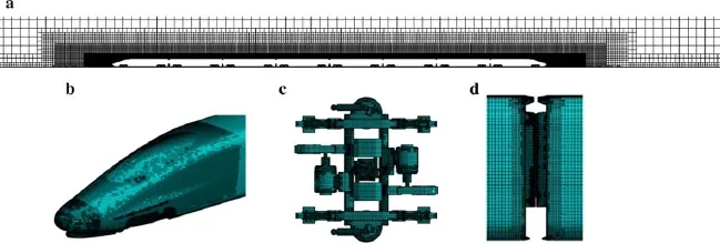
Fig.2　Computational mesh.a Section mesh in symmtry plane.b Train head surface mesh.c Bogie surface mesh.d Windshield surface mesh

Free-stream boundary conditions are applied to the inlet, exit,top,and side boundaries of the computational domain. Theno-slipwallboundaryissetforthegroundwithamoving velocity identical to the running speed of the train,which is 97.22 m/s（350 km/h）.The turbulent initial conditions are based on a synthetic eddy method,the turbulence intensity is 0.01,and the turbulent length scale is 0.01 m.

4　Validation

Experimental measurements were performed to validate the meshstrategyandthenumericalmethod.Thetestmodelused in the measurement is a 1/8th scaled model of the modifie CRH380A train with a 3-car grouping,including the train head,intercar,and train tail,and the length of the model is 9.75m.TheexperimentwasconductedattheShanghaiAutomotive Wind Tunnel Center in Tongji University.The free stream velocity is 60 m/s.The mesh strategy and numerical methodutilizedinthevalidation arethesameasdescribedin Sect.3,and the total number of mesh cells is approximately 24 million.The experimental setup in the wind-tunnel and the mesh of the model are shown in Fig.3a,b.The positions of the pressure monitors on the head train surface are shown in Fig.4 and are located on the symmetry plane of the model.The same monitor distributions can be found for the tail train in reverse sequence.The numerical results are the time-averaged values over a 2 s period after the flws are fully developed and are normalized by the free stream reference values.It can be seen that the numerical predictionsare in good agreement with the experimental values,which indicates that the mesh strategy and numerical method used in this paper are reasonable（Fig.5）.

Fig.3 a Photograph of wind tunnel model.b Surface mesh of train model and ground

Fig.4 Schematic diagram of measuring point

Fig.5 a Comparison between experimental and numerical results in train head.b Comparison between experimental and numerical results in train tail

5　Results and discussion

Thepurposeofthisstudyistoanalyzetheeffectsofthelength of a train and the affiliate components on train wind.The resultsarepresentedintwosections.First,thecharacteristics oftrainwind areanalyzed whensimplifie trainmodels with 3-,8-,and 16-car groupings are used.In the second section, the characteristics of train wind are analyzed when real train models are used.The effect of the affiliate components on train wind is analyzed by a comparison between the simplifie and real train models.Owing to the high unsteadiness of theflws around the trains,thevelocity ofthe trainwind will be presented with the time-averaged values over a 2 s period.

5.1Characteristics of train wind for simplifie train model

In this study,the train is stationary when the flw fielis calculated,thefreestreamandthegroundhavethevelocityof arunningtrain,andtherefore,whenanalyzingthetrainwind, stationarygroundshouldbetakenasthereferenceframe.The reference frame is established as follows:the direction of the train movement is the x-axis positive direction,the left side of the train movement is the y-axis positive direction,and the z-axis is determined in accordance with a right-handed coordinate system.The coordinates of the tip of the train’s leading nose are x=−39 m,y=0 m,and z=1 m.The length of the streamline shape of the train head is 12 m.

Fig.6　Contours of velocity of transverse train wind（TTW）and longitudinal train wind（LTW）in plane z=0.2 m and z=1.4 m

Whenthetrainmovesahead,theairflwaheadoftheleadingnoseispushedforwardandlaterally,airflwsthatarejust upstream and transverse change dramatically because of the cross-sectional shape ofthevarying trainhead.Inthemiddle of the train,the cross-sectional shape of the train remains constant,and the airflw changes slightly.In the train’s trailingnoseregionandwakeregion,sincetheairflwisaffected by the separated and detached flw near the trailing nose and the counterrotating vortices behind the trailing nose,the airflw changes dramatically,too.

In Fig.6,the longitudinal（train movement direction）and transverse velocity of airflw around the train in the plane z=0.2 m and z=1.4 m are shown.It can be seen that the train wind changes dramatically in the nose and wake regions.In Fig.7,the longitudinal and transverse velocities of train wind along the train length are illustrated at 3.0 m from the center of the train at different distances from the ground.The measuring position is based on BS EN 14067. It can be seen that the maximum longitudinal train wind （LTW）is below the maximum transverse train wind（TTW）. The train wind in a lower position is greater than that in a higher position.In the case of TTW,when the train is passing,the train wind velocity ahead of the tip of the leading nose increases dramatically along the train,then decreases behind the leading nose.The maximum velocity of the TTW appears at the position x=−38 m,which is 1 m behind the leadingnose.TheTTWisapproximately 0m/sinthemiddle of the train.In the train’s trailing nose and wake regions,the airflw is sucked toward the trailing nose,and the maximum TTWappearsatthepositionx=36m,whichis3maheadof the trailing nose.In the case of LTW,the train wind velocity increases and then decreases dramatically in the nose region. Two peaks can be observed sequentially for the leading nose region,a positive peak and a negative peak.As for the former,the velocity of the train wind increases in the running direction,reaches its maximum at the tip of the leading nose, and then decreases dramatically.As for the latter,the airflw runs in the opposite direction of the train and reaches its maximum around the streamline,while the converse is true in the trailing nose and wake regions.The maximum LTWappears at the position x=40（1 m behind the tip of the trailing nose）.The train wind in the transverse direction is greater than that in the longitudinal direction.Especially in the leading nose and trailing nose regions,a relatively large train wind appears.The variation in the cross section of the streamlinedshapecoulddrawinastrongertrainwind.Forthe position 3 m away from the train center,the boundary-layer effectseemstoinfluenc thetrainwindtoalesserextent.For the simplifie train model,the train wind caused by the leading nose is slightly greater than that caused by the trailing nose.

Figure 8 shows the variation in the train wind direction at 3.0 m from the COT at 0.2 and 1.4 m high from the ground along the train length.It can be seen that the directions are outward along the leading streamline,backward along the trainbody,andinwardandforwardalongthetrailingstreamline.

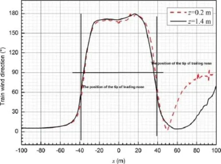
Fig.8　Train wind direction at 3.0 m from COT at different heights from ground along 3-car group simplifie train length

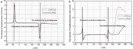
Fig.9　a TTW of 8-car group simplifie train along train length.b LTW of 8-car group simplifie train along train length

Figures 9 and 10 show the LTW and TTW along the train length illustrated at 3.0 m from the COT at different distances from the ground for 8-car group and 16-car group trains.It can be seen that regardless of the LTW or the TTW in the upstream,the same spatial distribution is retained as that of 3-car group train.The magnitude of the train wind remains the same too.The magnitude of the TTW in the downstream remains the same as that of the 3-car group train.The TTW mainly relates to the streamlined shape, seldom to the length of the train.However,the LTW apparently varies for trains with different groups.The maximum LTW reaches 3.5 m/s for a 3-car group,while it is 16.4 and 16.2 m/s for 8-car and 16-car group trains,respectively.This is a result of the development of a boundary layer along the train length.Different lengths of trains lead to different thicknesses of the boundary layer in the downstream, which also leads to different states of trailing vortices.As shown in Fig.9,a line located 3 m from the train axis is very close to the edge of the boundary layer of the flw,and it comes into the boundary layer at x=140 m.As a result, a stronger longitudinal train wind can be observed in these places.

Figure 11 shows the variation in the train wind at lines along the train length ranging from 1.7 to 4.2 m from the COT at a height of 1.4 m from the ground.It can be seen that the LTW is almost the same before the streamlined head for different lines varying considerably in the downstream direction.For a line of y=1.7 m,it is just 0.01 m from the train side surface and completely inside the boundary layer, which results in a stronger LTW.Because of the sharp variation in the shape at the connection between the streamlined head and the train body,the maximum transverse train wind is observed here.With an increasing cross distance from the train side surface,the LTW begins to decrease.Meanwhile, the LTW tends to be stronger in the downstream direction owing to the boundary-layer effect.Velocity profile at dif-ferent positions along the train body are shown in Fig.10b, in which the x-coordinate denotes the normal distance along the train axis.It can be seen that the longitudinal velocity is increased as the position goes backward,indicating that the boundary layer thickens in the downstream direction.

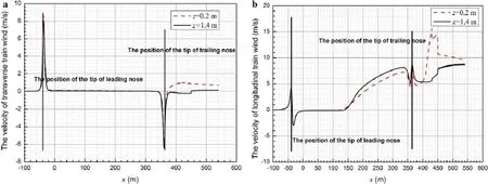
Fig.10　a TTW of 16-car group simplifie train along train length.b LTW of 16-car group simplifie train along train length

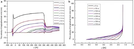
Fig.11　a LTW of 16-car group simplifie train along train length at different distances from COT at z=1.4.b LTW distribution at different positions along train length at z=1.4 m

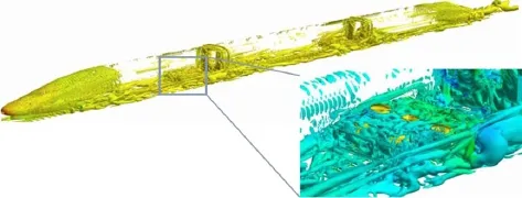
Fig.12　Isosurface of Q around train flw fiel

It can be concluded that a stronger train wind could be induced at the leading and trailing streamline.When a simplifie train model is adopted,the model with fewer groups could underestimate the magnitude of the train wind in the downstream direction.

Fig.13　Instantaneous velocity magnitude contour at different heights

Fig.14　Schematic diagram of relative train position

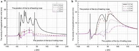
Fig.15　LTW distribution along real train length for 3-car group.a LTW distribution at y=1.8 m from COT.b LTW distribution at y=3.0 m from COT

5.2Characteristic of train wind of real train model

When a simplifie model is utilized,except for the leading and trailing streamlines,the disturbance to the flw by the train body is very limited.However,when a real train is running,the components will cause a strong disturbance to the flw.These components consist of the bogies and the corresponding bogie cabins in the bottom,the windshields in the middle,and the pantographs on the top of the train.In this section,a real train model is adopted,and all the com-ponents are considered except for the pantographs,whose influencon the slipstream around the train body is less pronounced.

Fig.16　LTW distribution along real train length for 8-car group.a LTW distribution at y=1.8 m from COT.b LTW distribution at y=3.0 m from COT

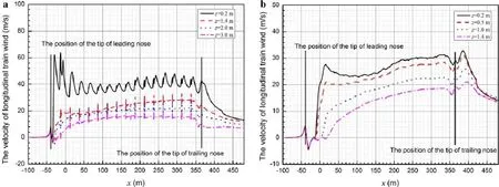
Fig.17　LTW distribution along train length for 16-car group.a LTW distribution at y=1.8 m from COT.b LTW distribution at y=3.0 m from COT

Figure 12 shows the isosurface of Q around the train.Q representsthesecond-orderinvariantofthevelocitygradient tensor and can be used to reveal the vortices in the flw field It can be seen that strong vortices exist at the bottom of the train,especially in the bogie regions.

Figure 13 shows the velocity contour at different heights around a high-speed train.It can be seen that the flw is disturbed strongly in regions around the bogies and windshields.When the train is running,the bogies and bogie cabins encounter flw around them,and flw inside the bogie cabin is brought about at high speeds.Owing to the sharp curvature of the windshields,flw is disturbed, and consequently the flw inside the boundary layer is changed.The flw is easily separated in the bogie zones, and strong vortices can be observed there.As a result, the surrounding train wind is strengthened.As the height increases,the train wind tends to weaken,which is a result of the relatively lower position of the bogie cover. However,compared to the simplifiemodel,the velocity distribution in the weak zone for the real train model is more complicated since the flw in the weak zone is more turbulent.

Considering the unsteady characteristics of the flw field the time-averaged train wind at 2 s is adopted when the train wind is analyzed.Figure 14 shows the positions of the train wind probes compared to the train.

Figures 15,16,and 17 show the distribution of the LTW along the train body at different heights for the 3-car,8-car, and 16-car group real train models.The exact positions of the nose tip for the leading and trailing cars are also depicted in the figure It can be seen that the velocity of the LTW is the same for high-speed trains of different groups in the zone around the leading nose.The train wind decreases as the height increases.Compared to the simplifie model,the distribution of wind around the leading nose is the same for the real train model,indicating that the bogie zones have little influenc on train wind in the upstream.After the flwpasses the leading streamline,it is disturbed by the bogies and the bogie cabins.As a result,the velocity distribution inside the boundary layer varies significantl.The difference increaseswhenapproachingtheground.Comparingthetrain modelswithdifferentgroups,themaximumtrainwindexists around the second bogie zone for a line of y=1.8 m and z=0.2 m.Meanwhile,the value of the maximum LTW is the same compared to each other（3-car,8-car and 16-car models）,since the train wind there is mainly a result of the flwfromthefirs andsecondbogiezones.Forthe y=1.8m sectionplane,astheheightincreases,thedevelopment ofthe boundary layer begins to dominate instead of the influenc of the bogie region.As the length of the train increases,the maximumvalueofthevelocityoftheLTWinthedownstream part of the train increases,and the maximum LTW exists at the trailing train body,which is just in front of the trailing streamline.

Fig.18　LTW distribution along real train length for 3-car group.a LTW distribution at different distances from COT at z=0.2 m.b LTW distribution at different distances from COT at z=1.4 m

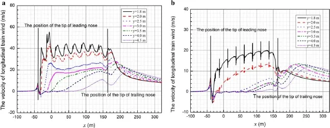
Fig.19　LTW distribution along real train length for 8-car group.a LTW distribution at different distances from COT at z=0.2 m.b LTW distribution at different distances from COT at z=1.4 m

Fig.20　LTW distribution along real train length for 16-car group.a LTW distribution at different distances from COT at z=0.2 m.b LTW distribution at different distances from COT at z=1.4 m

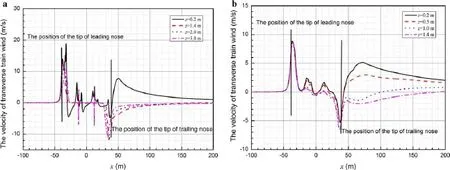
Fig.21　TTW distribution along real train length for 3-car group.a TTW distribution at y=1.8 m from COT.b TTW distribution at y=3.0 m from COT

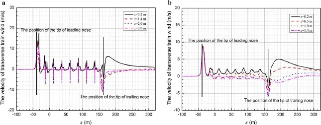
Fig.22　TTW distribution along real train length for 8-car group.a TTW distribution at y=1.8 m from COT.b TTW distribution at y=3.0 m from COT

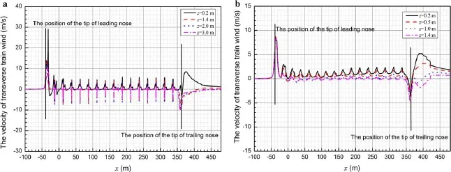
Fig.23　TTW distribution along real train length for 16-car group.a TTW distribution at y=1.8 m from COT.b TTW distribution at y=3.0 m from COT

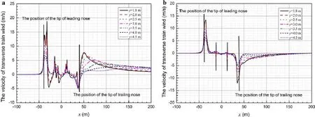
Fig.24　TTW distribution along real train length for 3-car group.a TTW distribution at different distances from COT at z=0.2 m.b LTW distribution at different distances from COT at z=1.4 m

Fig.25　TTW distribution along real train length for 8-car group.a TTW distribution at different distances from COT at z=0.2 m.b LTW distribution at different distances from COT at z=1.4 m

Forplacesfarfromthecentrallineofthetrain（y=3.0m, for instance）,the influenc of the bogie zone becomes limited.Compared to the simplifiemodel,the LTW in the downstreampartoftherealtrainmodelgrowsmuchstronger for a line of y=3.0 m and z=0.2 m.At a position of y= 3.0 m and z=1.4 m,it will easily enter the boundary layer owing to the influenc of the windshields and bogies.Consequently,a strong LTW is observed.This position is nearly outside of the boundary layer for the case of the 3-car group train.For the case of an 8-car group train,this line enters the boundary layer at x=140 m for the simplifie model and at 75 m for the real train model.For the case of a 16-car group, the entry spots are the same as with the 8-car group.AnalyzingthedistributionoftheLTWinthewakezone,asignifican difference can be observed for the simplifie model and the real train model,indicating that the structures at the bottom of the train greatly influenc the flw status in the wake zone.

Figures 18,19,and 20 show the distributions of the LTW along the train body at different distances from the central line of the train and different heights.For the z=0.2 m section,the tendency is the same for trains with different size groups.As the distance from the central line of the train increases,the LTW decreases.For the position close to the central line,the maximum LTW occurs at the middle of the train.However,as the distance increases,the maximum LTW occurs in the wake zone.For the z=1.4 m section,the distribution of the longitudinal train wind along themiddlepartofthetrainisthesameasinthelowersection. However,the maximum LTW of the train with 16 groups is significantl higher than that of the train with 3 groups.It can also be seen from the figure that a strong influenc from the windshields is observed in the y=1.8 m section.

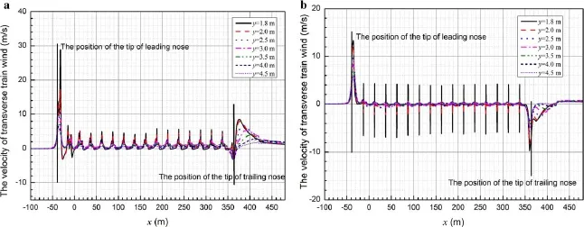
Fig.26　TTW distribution along real train length for 16-car group.a LTW distribution at different distances from COT at z=0.2 m.b LTW distribution at different distances from COT at z=1.4 m

Table 1　Maximum magnitude of train wind for different models

As discussed earlier,an obvious difference exists for the LTW along the train length between the simplifie train and real train models.Moreover,as the group number grows,the maximum LTW increases for the real train model.

Figures 21,22,and 23 show the TTW for trains with different size groups.It can be seen that the place where the maximum TTW at the same height occurs is the same for trains with different size groups,as is the magnitude of the TTW.The maximum TTW decreases as the height increase in the y=1.8 m section.For a line of y=1.8 m and z=0.2 m,the maximum TTW of the real train model emerges at x=−32 m,which is just behind the firs bogie, withamagnitudeof18m/s.Astheheightincreases,theTTW at different heights coincides along the train body except for the leading and trailing streamlines.This is because of the limited influenc of the bottom bogies.However,for the of y=3msection,whichisalittlefarfromthebogiecover,the streamlinedshapeisthemainfactorthatinfluence theTTW. Thestreamlineofthetrainisakindofslenderbodythatleads to the same position for the maximum TTW.The maximum TTW occurs at x=−37 m with a value of 8.5 m/s.Because of the constant area of the cross section of the train body in the middle,the magnitude of the TTW is very close to zero.Although the boundary layer develops along the train body,the influenc on the TTW from the variation of the boundary layer is very slight.In addition,the influenc of the windshield is also very slight.

Figures 24,25,and 26 show the distributions of the TTW along the train body at different distances from the central line of the train and different heights.It can be seen that the TTWaroundtheleadingstreamlinedecreasesasthedistancefromthecentrallineofthetrainincreases.Inthemiddleofthe train,takingthesectionofz=0.2masanexample,theinflu enceofthebogiesdiminishesasthecrossdistanceincreases. For the z=1.4 m section,the influenc of the windshields diminishesasthecrossdistanceincreases.Meanwhile,inthe wake zone of the train,it can be observed that the TTW is not affected by the length of the train.For the z=0.2 m section,the flw is pushed away by the bogie,which leads to a relatively stronger outward TTW.For the z=1.4 m section, which is far from the bogies,the TTW is mainly affected by thetrailingvorticesinthewakezoneandgoesinwardtoward the train.

As discussed earlier,the TTW is mainly affected by the streamlinedshape,thebogies,andthewindshields.However, it is not affected at all by the length of the train.

Table 1 shows the maximum train wind magnitude in different regions at different heights with different groups. It can be seen that the maximum train wind magnitude in the leading streamline region is almost the same for different groups and different models（simplifiemodel or real train model）.In the middle region,owing to the influenc of the bogies and windshields,the thickness of the boundary layer varies.Consequently,the maximum train wind clearly varies.In the wake zone,the maximum train wind differs as well.Taking the case of the 3-car group model at the line of y=3 m and z=1.4 m as an example,the maximum train wind magnitude for the simplifie model occurs in the leading streamline region and in the wake region for the real train model;this is true in the case of eight groups as well. However,for the case of the 16-car group model,the maximum train wind magnitude for the simplifie model occurs in the wake region and in the middle region for the real train model.

6　Conclusions

This study evaluates the influence of affiliate components andlengthontrainwindusinganIDDESmethod.Theresults can be presented as follows:

（1）In the region ahead of the leading nose,the affiliate components and length of the train have no effect on train wind.Train wind is only a function of the streamline shape of the train nose and the running speed of the train.

（2）The length of the train affects the development of the boundary layer:the longer the length of the train,the thicker the boundary layer in the rear part of the train, whichstrengthenstheLTWat3.0mfromthecenterline of the train at different heights from the ground parallel to the train length.The development of the boundary layer has no effect on the TTW,which is only related to the streamline shape.

（3）Affiliate components,suchasbogies,bogiecabins,and windshields,affect the flw fiel in the near fiel of the train.Bogies andbogie cabins strengthen thetrain wind near the ground,and the train wind in the windshield region will be disturbed greatly by the windshields.

（4）The distribution of the LTW for a real train is different from that of the simplifie model.The velocity of the LTW in the rear part of the real train model is higher than that of the simplifie train model.As the train length increases,the maximum value of the LTW increases.

（5）Thetrainwindwillbeunderestimatedwhenasimplifie or short-group train model is used.A real train model with an 8-car grouping is adequate for the evaluation of train wind.

References

1.Baker,C.J.,Sterling,M.,Figura-Hardy,G.,etal.:Theeffectoftrain slipstreams on passengers and trackside workers.In:Proceedings of the 7th World Congress on Railway Research,Monteral,2006

2.Pope,C.W.:EffectiveManagementofRiskfromSlipstreamEffects atTracksideandPlatforms.RailSafetyandStandardsBoard-T425 Report,2007

3.Gilbert,T.,Baker,C.J.,Quinn,A.:Gusts caused by high-speed trains in confine spaces and tunnels.J.Wind Eng.Ind.Aerodyn. 121,39-48（2013）

4.Baker,C.:The flw around high speed trains.J.Wind Eng.Ind. Aerodyn.98,277-298（2010）

5.Baker,C.J.,Quinn,A.,Sima,M.,etal.:Full-scalemeasurementand analysisoftrainslipstreamsandwakes.Part1:Ensembleaverages. Proceedings of the Institution of Mechanical Engineers,Part F: Journal of Rail and Rapid Transit 228,451-467（2014）

6.Yao,S.,Sun,Z.X.,Guo,D.L.,et al.:Numerical studies on wake characteristics of high-speed trains.Acta Mech.Sin.29,811-822 （2013）

7.Muld,T.W.:Slipstream and flw structures in the near wake of high-speed trains［Ph.D.Thesis］Stockholm:KTH Aeronautical and Vehicle Engineering,2012

8.Liao,S.,Mosier,P.,Kennedy,W.,et al.:The aerodynamic effects ofhigh-speedtrainsonpeopleandpropertyatstationsintheNortheast Corridor.US Department of Transportation Federal Railroad Administration,1999

9.Lei,B.,Liu,Y.-G.:Computational analysis on human body aerodynamic force due to train induced air flw.J.China Railw.Soc. 21,20-23（1999）

10.Huang,Y.,Wu,W.,Zhang,H.,et al.:Discrete vortex method and its engineering application.J.Basic Sci.Eng.8,4（2000）

11.Tong,B.,Xia,N.,Li,Q.:Dicrete-vortex method in external flw problems.Adv.Mech.15,318-328（1985）

12.Li,R.,Zhao,J.,Zhang,S.,et al.:Influenc of the aerodynamic force to human body near high-speed trains.China Railw.Sci.28, 22（2007）

13.Hemida,H.,Baker,C.:The calculation of train slipstreams using large-eddy simulation techniques.In:9th World Congress on Railway Research,Lille,22-26 May,2011

14.Hemida,H.N.:Large-eddy simulation of the flw around simplifie high-speed trains under side wind conditions.［Ph.D.Thesis］Chalmers University of Technology,Goteborg（2006）

15.Lee,H.:Assessment of potential aerodynamic effects on personnel and equipment in proximity to high-speed train operations. US Department of Transportation Federal Railroad Administration,1999

16.Peng,L.-M.,Liu,C.,Shi,C.-H.,et al.:Characteristics of the train wind and analysis of personnel safety in the high-speed railway station.J.Zhengzhou Univ.（Eng.Sci.）34,99-102（2013）

17.Star CCM+User Guide version 9.04,CD-adapco Corporation

30 July 2015/Revised:28 October 2015/Accepted:2 November 2015/Published online:17 March 2016

✉Dilong Guo

jack9517@126.com

1Key Laboratory for Mechanics in Fluid Solid Coupling Systems,Institute of Mechanics,Chinese Academy of Sciences,No.15 Beisihuanxi Road,Beijing 100190, China

2CSR Qingdao Sifang Co.Ltd.,Qingdao 266111, China