Accurate disparity estimation in light field using ground control points
2016-07-19HaoZhuQingWangcTheAuthor206ThisarticleispublishedwithopenaccessatSpringerlinkcom
Hao Zhu,Qing Wang()?cThe Author(s)206.This article is published with open access at Springerlink.com
Research Article
Accurate disparity estimation in light field using ground control points
Hao Zhu1,Qing Wang1()
?cThe Author(s)2016.This article is published with open access at Springerlink.com
1School of Computer Science,Northwestern Polytechnic University,Xi’an 710072,China.E-mail:qwang@ nwpu.edu.cn().
Manuscript received:2015-12-01;accepted:2016-04-01
AbstractThe recent development of light field cameras has received growing interest,as their rich angular information has potential benefits for many computer vision tasks.In this paper,we introduce a novel method to obtain a dense disparity map by use of ground control points(GCPs)in the light field. Previous work optimizes the disparity map by local estimation which includes both reliable points and unreliable points.To reduce the negative effect of the unreliable points,we predict the disparity at non-GCPs from GCPs.Our method performs more robustly in shadow areas than previous methods based on GCP work,since we combine color information and local disparity.Experiments and comparisons on a public dataset demonstrate the effectiveness of our proposed method.
Keywords disparity estimation;ground control points (GCPs);light field;global optimization
1 Introduction
Withtherapiddevelopmentofcomputational photography,manycomputationalimaging deviceshavebeeninvented, basedon, e.g.,coded apertures[1],focal sweep[2],and light fields[3,4],examples of the latter being the Lytro (https://lytro.com) andRaytrix(http://www. raytrix.de)cameras.As a light field camera captures both spatial and angular information about the distribution of light rays in space,it provides a potential basis for many fundamental operations in computer vision[5-8].In this paper,we focus on accurate disparity estimation using the light field.
Disparity estimation in stereo[9-11]is a longstanding problem in computer vision,and it plays an important role in many tasks.Given two or more images captured from different viewpoints,the fundamental problem is to find the optimal correspondence between these images.Unlike the point information captured by a traditional camera,a light field camera captures information about the light,providing a full description of the real world via a 4D function.We can obtain so-called subaperture images[12],and synthesize a multi-view representation of the real world.Unlike the wide baseline used in traditional multi-view stereo,the multi-view representation synthesized by the light field has a narrow baseline,which can provide more accurate sub-pixel disparity estimation.
Previous work[13,14]has computed an optimized disparity map based on local estimation,which includes both reliable and unreliable information. Undoubtedly,reliable points will have a positive effect on the global disparity map,but the effect of unreliable points may be detrimental.To reduce the negative effects of unreliable points,we propose to obtain a dense disparity map from certain reliable estimation points in the light field called groundcontrolpoints(GCPs)[15].GCPsare sparse points which can be matched reliably in stereo,and are often obtained by stable matching or laser scanning.We determine GCPs by the reliability of the structure tensor,and construct the GCP spread function based on color similarity and local disparity similarity.By combining local disparities,the proposed method performs more robustly than the previous GCP method in shadow areas:experimental results on the LFBD dataset[16]show that our method performs more robustly than the original light field method[14]and the originalGCP method[15].
The rest of this paper is organized as follows. In Section 2,we review the background and prior work on depth estimation from a light field and the GCP method.Section 3 describes our algorithm. We give the experimental results in Section 4,and our conclusions and suggestions for future work are provided in Section 5.
2 Background and related work
A light field[17]is represented by a 4D function f(x,y,u,v),where the dimensions(x,y)describe the spatial distribution of light,and the dimensions (u,v)describe the angular distribution of light. When we fix one spatial dimension y∗and one angular dimension v∗,we get the epipolar plane image(EPI)[18](see Fig.1).
In a rectified EPI,the slope k of a line has a linear relationship with the depth d(see Fig.2),the larger the depth,the larger the slope:d=fsk/c,where f is the focal length of the lens,s is the baseline between the two views,and c is the pixel size.Given the EPI structure,the depth estimation problem is converted into a slope detection problem.As light field cameras capture angular information,analyzing the EPI is a suitable way to estimate depth using the light field.

Fig.1 The epipolar plane image obtained by fixing one spatial dimension and one angular dimension.

Fig.2 Left:epipolar plane image.Note that the slope is the reciprocal of the disparity.Right:the inverse relationship between disparity and depth.The relationship between slope and depth is linear.
Structuretensor(ST).Wannerand Goldluecke [14]proposedtoanalyzetheEPI by the structure tensor,obtaining the local disparity andthecorrespondingreliabilityatthesame time.They then optimized the local disparity map by a global energy function based on variational regularization.However,as they pointed out,the sampling of viewpoints must be dense enough to guarantee that the disparity between two views is less than 2 pixels,otherwise the straight line will become a broken line in the EPI,leading to inaccurate local estimation.This issue will be discussed in Section 3.1.
Lisadtransform.TosicandBerkner [19]proposed the light field scale and depth transform. Theyinitiallydetectedtheslopeoftheepitube[20]in Lisad-2 space,and then repaired depth discontinuous areas using the slope of the epistrip[20]detected in Lisad-1 space.
Multiple cues.Tao et al.[21]proposed a method to estimate depth by combining multiple cues,including correspondence cues and defocus cues.The advantages of using different cues in different areas were exploited,and they obtained good results for real scenes.
RPCA(robustprinciplecomponent analysis) matching.HeberandPock[22]considered the highly redundant nature of the light field,and proposed a new global matching term based on low rank minimization.Their method achieves the best results on synthetic datasets.
GCP method.Ground control points are sparse points which can be matched reliably in stereo. Wang and Yang[15]proposedto predict the disparity of non-GCPs from GCPs,and optimized the initial disparity map using a Markov random field(MRF)energy function containing three terms: a data term,a smoothness term,and the GCP term. The top ranking results achieved on the Middlebury dataset prove that it is a good approach to stereo matching.However,it performs poorly in shadow (see Fig.5)as it assumes that two points with similar colors should have similar disparities,but the colors may differ between a center point and its neighbors while their disparities are similar.
3 Theory and algorithm
3.1Algorithm overview
Our approach is given in Algorithm 1.The inputis the 4D light field L(x,y,u,v)and the reference view index r.The output is the disparity map D. The algorithm consists of five steps:
1.Local estimation.The local disparity map and its reliability map are obtained by using the structure tensor method(see Section 3.2).
2.GCP detection.The most credible points as determined by the reliability map are selected as the GCPs(see Section 3.2).
3.GCP optimization.The GCP spread function is built using the local disparity map and the set of GCPs.By using this function,intermediate results are obtained(see Section 3.3).
4.Building the energy function.The intermediate results from GCP optimization are combined with traditional stereo matching function results (see Section 3.4).
5.Final optimization.The energy function is found by optimization(see Section 3.4).
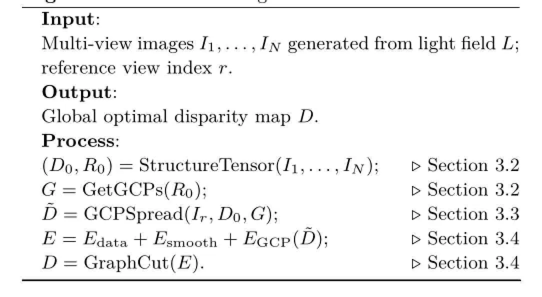
Algorithm 1:Our GCP algorithm____________________
3.2Local disparity and GCPs
We use the structure tensor to detect the slopes of lines in the EPI:
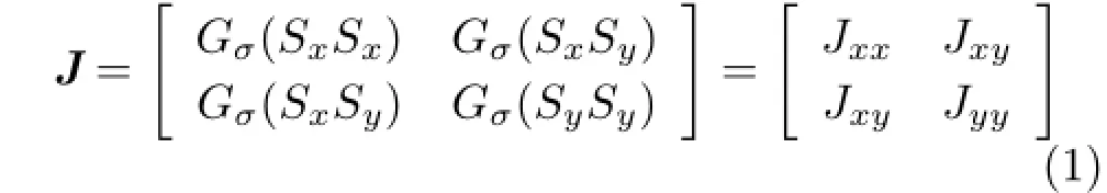
where Gσrepresents a Gaussian smoothing operator,and Sx,Syrepresent the gradients of the EPI in x and y directions respectively.
Then,the direction of the line is
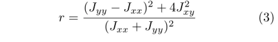
and its reliability is measured by the coherence of the structure tensor:
It is worth noting that the structure tensor performs poorly in the near field(see Fig.4),which corresponds to the low-slope area in the EPI;in other words,the disparity between two views is larger than 2 pixels in these areas.We adopt the easiest method to solve this issue-by scaling up the EPI along the y axis in these areas to convert the low-slope area into a high-slope area.We use bicubic interpolation to scale up the EPI.After calculating the slope of the scaled EPI,we can recover the slope of the original EPI by dividing by the scaling factor.An original EPI and the scaled up EPI can be seen in Fig.3.The improvement of our method can be seen in Fig.4.
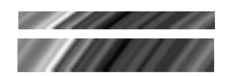
Fig.3 Top:an original EPI.Bottom:the scaled up EPI.Clearly,the slopes of the lines are greater in the latter.
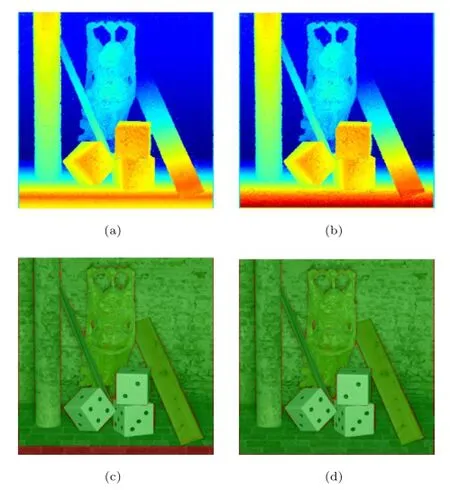
Fig.4 Disparity and error map obtained by the basic structure tensor method and our method for the Buddha dataset.(a)Disparity map obtained by the basic structure tensor method.(b)Disparity map obtained by our improved method.The basic structure tensor method performs poorly at close range.(c)and(d)Relative depth error maps for the above two methods.Relative depth errors of more than 1%are indicated in red.The error rates of these two methods are 7.87%and 3.97%,respectively.
Having obtained the coarse disparity map D0and its reliability map R0from the structure tensor,it is unnecessary to do stable matching or laser scanning to obtaining GCPs;to do so would be timeconsuming and laborious.We obtain the set of GCPs G from the reliability map R0.
3.3GCP spread function
The inputs to our GCP spread function are the reference view image Ir,the local disparity map D0,and the set of GCPs G.
Unlike Wang and Yang’s method[15],which constrains similar colors to have similar disparities,we use the constraint that two neighboring pixels p and q should have similar disparities if not only their colors are similar but also their local disparities are similar.This constraint can be described by minimizing the difference between the disparity of p and a weighted combination of its neighbors’disparities.The global cost function is given by

where∆Cpqand∆D0,pqarerespectivelythe Euclidean distances between pixels in RGB color space and local disparity(D0)space.Parameters γc,γd,and?control sharpness of the function.To ensure that the disparity term and the color term have the same order of magnitude,the parameter γdis not independent,and is calculated from the following equation:
where Cmaxand Cminare the maximum and minimumvaluesincolorspace,255and0 respectively.NCis the number of color channels,here 3.Parameters dmaxand dminare the maximum and minimum values in hypothetical disparity space,respectively.sγdis a weight to control the strength of the disparity term.We suggest that the disparity term should be larger than the color term,so sγd<1.
Equation(4)is a quadratic function.After taking its derivative to find the extremum,we find that the disparity of the center point p has a linear relationship with the disparities of its neighbors:
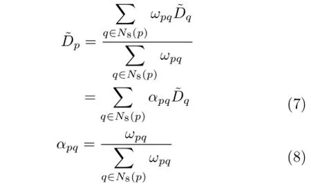
Given the linear relationship above,we can derive the disparity of non-GCPs from GCPs by solving a system of sparse linear equations(I-A)x=b,where I is an identity matrix,and A is an N×N matrix(N is the number of points in the image).In each row of A,if the corresponding pixel p belongs to the GCPs,all elements are zero,otherwise only the 8-connected neighbor points q have non-zero values,equal to their weights αpq.Similarly,for the elements in vector b,only the pixels belonging to GCPs have non-zero values,and are equal to their initial disparities.x is the optimal disparity map that we hope to obtain.
3.4Energy functions with the GCPs
Our energy function contains three terms:a data term,a smoothness term,and the GCP term.
As the length of the baseline between two views in the light field camera is narrow,we combine the basic sum of squared differences(SSD)and sum of squared gradient differences(SSGD)as our data term to ensure good matching: and

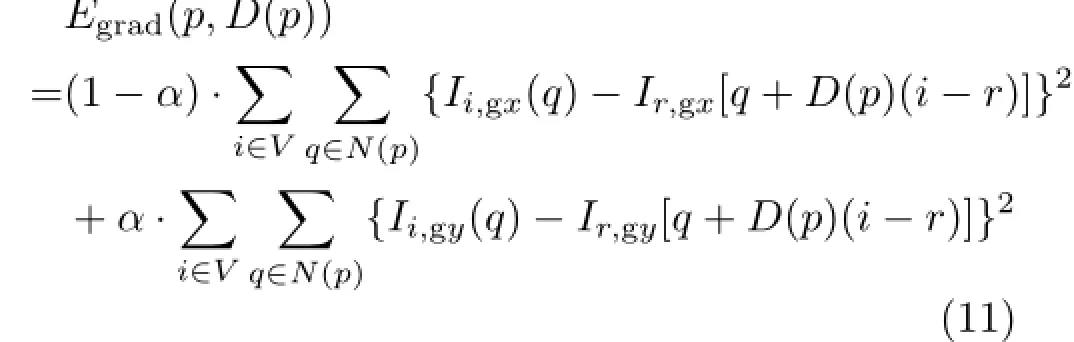
Here,D is the global optimal disparity map,D(p)is the disparity value of point p,V is the number of views in the light field,N(p)is an image patch centered at pixel p,Iris the reference view in the light field,and Ii,gxand Ii,gyare the gradients of the i-th view image in x and y directions,respectively.
We select the widely used linear model based on a 4-connected neighborhood system as our smoothness term,which is expressed as
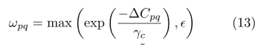
where∆Dpqis the difference in disparity between pixels p and q,λsis a smoothness coefficient to control the strength smoothing,and ωpqis a weight based on the distance between p and q in RGB color space:
Given the optimal disparity˜Dpobtained by the GCP spread function in Eq.(7),we can now employ the robust penalty function[15]:

where λris a regularization coefficient that controls the strength of the GCP energy;γdand η control the sharpness and upper-bound of the penalty function.
4 Experimental results
4.1Parameters and dataset
In our experiments,we have found that the structure tensor method performs poorly for lines in the EPI with slope larger than 0.65.So,we first analyze the EPI by structure tensor,and then if the slope of 50% of points is larger than 0.65,we scale this EPI from 9 to 17 pixels in the y direction,and reanalyze the EPI.
We set two thresholds to select GCPs,using absolutereliabilityandrelativereliability. The absolute reliability is set to 0.99 in our implementation.If the reliability of a point is larger than 0.99,it is classified as a GCP.If only this criterion is used,GCPs may be too sparse in some datasets to reliably determine the disparity map calculated from the GCPs.We thus also consider relative reliability.If the fraction of GCPs obtained by considering absolute reliability is smaller than a set percentage(20%),we select the 20%most relaible points as GCPs.
For the disparity map obtained from GCPs,the parameters γcand?are set to 30 and 0,respectively. The weight parameter sγdis set to 0.25.Note that if γcor γdis unsuitable,the sparse linear system may be singular.
In the data term,the parameter α is set to 0.5,and the size of image patches is 7×7.The parameters γcand?in the smoothness term are set to 3.6 and 0.3,respectively.And the parameters η and γdare set to 0.005 and 2 according to Wang and Yang[15],respectively.In the final energy function,the smoothness coefficient λsand the GCP scaling coefficient λrare set to 1.67 and 4.67,respectively. We divide the disparity into 120 levels,and use linear interpolation to get floating point values for use in the data term.We use GCO-v3[23-25]to optimize our energy function.
We tested our method using HCI LFBD [16],which contains synthetically generated light fields,each of which is represented by 9×9 sub-aperture images.The dataset was rendered by Blender (http://www.blender.org),and contains the ground truth.
Our algorithm was implemented in MATLAB,on MacOS X 10.11.1 with 8 GB RAM and a 2.7 GHz processor.The running time for a 9×9×768×768×3 light field is 60 minutes.Most of the cost is to build two large sparse matrices for the smoothness term and the GCP term,and could be greatly reduced by reimplementation in C.
4.2Comparision with previous works
We compare our GCP propagation method with the basic structure tensor method and Wang and Yang’s method[15]in Fig.5.Our method performs more robustly than Wang and Yang’s in shadows and in color discontinuous areas.
We also compare our results with Wanner and Goldluecke’s[14]and Wang and Yang’s[15]results,as shown in Fig.6.Note that there is much noise in the initial map;there is reduced noise after the GCPs’spread.A quantitative comparison can be seen in Table 1.We select the relative depth error as our criterion(we used 0.2%here). Our method performs better than Wanner and Goldluecke’s on 4 datasets,but worse on 3 datasets. On analyzing these 7 datasets we find that there arefewtransparentmaterialsintheBuddha,StillLife,Horses,and Medieval datasets,but more transparent materials and shadows,lamps,and mirrorsintheBuddha2,Mona,andPapillondatasets.Stereo matching outperforms the structure tensor method in a Lambertian environment,whilst thestructuretensorperformsbetterinnon-Lambertian environments.
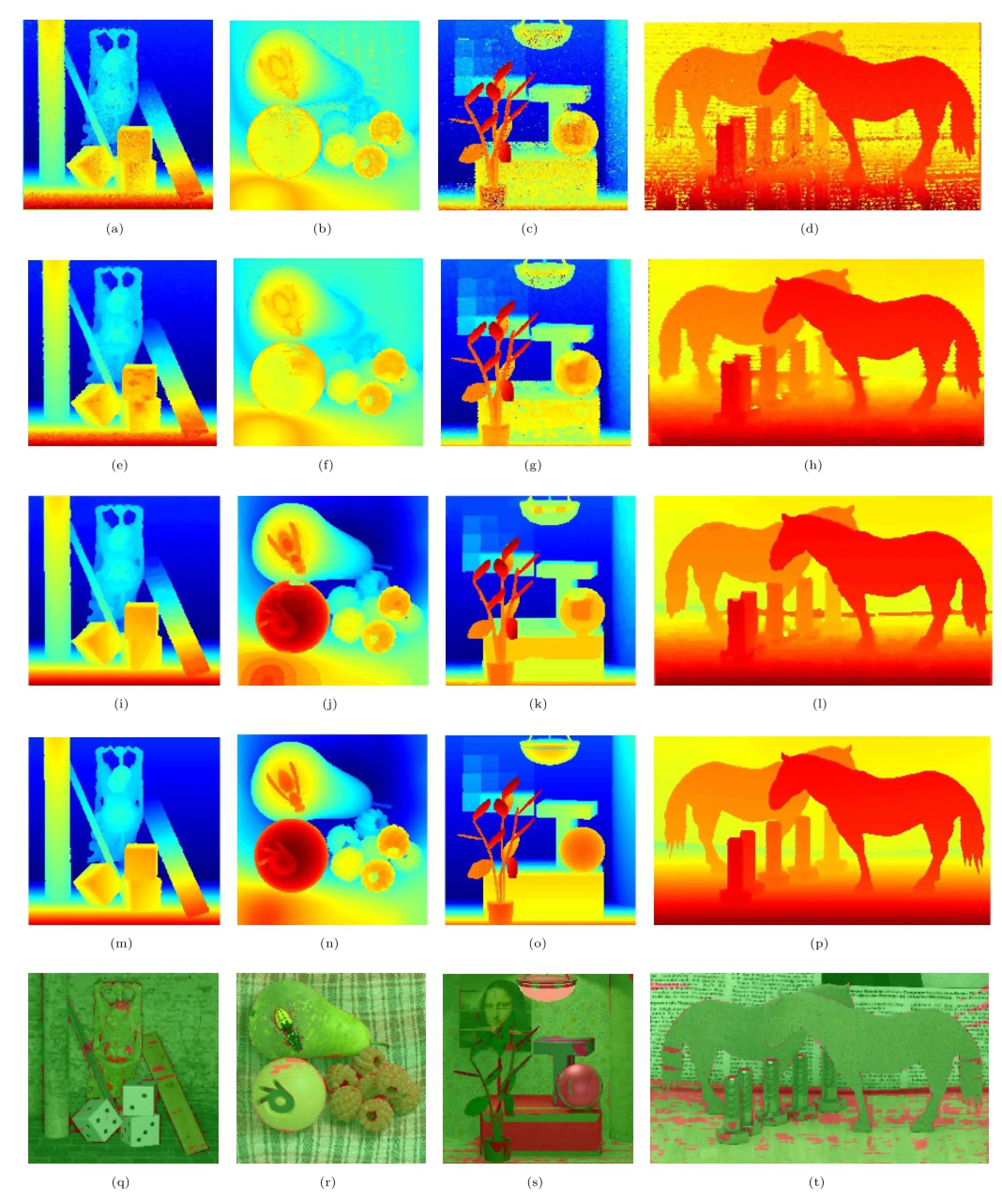
Fig.6 Results of our method on Buddha,StillLife,Mona,and Horses datasets from LFBD.Top:initial disparity map D0.2nd row:results ˜D from the GCP spread function.3rd row:final results of our method.4th row:ground truth.Bottom:error map.Relative depth errors of more than 0.2%are shown in red.
Our method performs better than Wang and Yang’s method,especially for the Papillon,StillLife,and Horses datasets.Note that there exist some shadows in these datasets;the disparities of shadow areas ought to be the same as those of their neighborhoods.As local disparity information is combined in our GCP spread function,our method outperforms Wang and Yang’s.
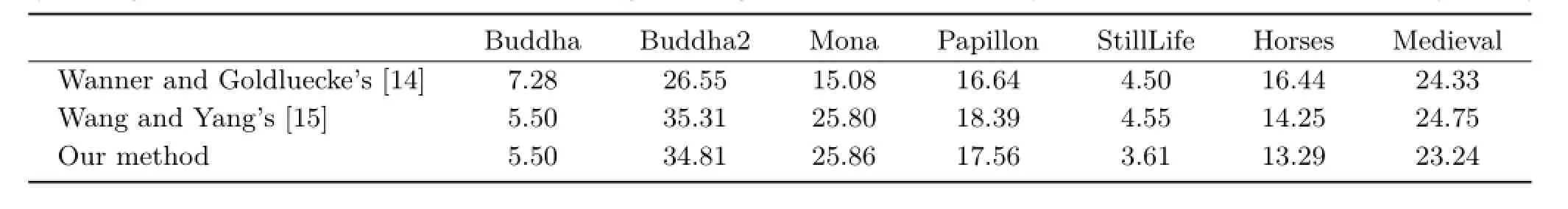
Table 1 Percentage of pixels with depth error more than 0.2%for LFBD[16].The results of Wanner and Goldluecke’s method were obtained by running their public source code.The results of Wang and Yang’s method were obtained by our implementation (Unit:%)
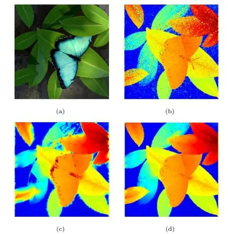
Fig.5 Comparison.(a)Input dataset;there are two colors in the butterfly and a shadow on the leaves to the left of the butterfly.(b)Basic structure tensor result,showing many points with wrong values. (c)Wang and Yang’s propagation strategy assigns wrong disparities to shadow areas and divides the butterfly into 2 parts along the color boundary in its tail.(d)Result of our GCP propagation method,with few wrong values and good performance in shadow areas.
5 Conclusions and future work
In this paper,we have proposed the idea to determine GCPs by using the reliability of the structure tensor. We also give a more robust GCP spread function than Wang and Yang’s[15]to propagate disparity from GCPs to non-GCPs.Experimental results on LFBD show that our method performs more robustly than Wanner and Goldluecke’s and Wang and Yang’s methods.However,our method performs less well in strong light and complicated shadow areas;this is a problem for most stereo methods.In the future,we will continue to investigate stereo in light fields,and take the advantages of more features of light field to solve these problems.
Acknowledgements
The work was supported by National Natural ScienceFoundationofChina(Nos.61272287,61531014)and a research grant from the State Key Laboratory of Virtual Reality Technology and Systems(No.BUAA-VR-15KF-10).
References
[1]Levin,A.Analyzing depth from coded aperture sets. In:Lecture Notes in Computer Science,Vol.6311. Daniilidis,K.;Maragos,P.;Paragios,N.Eds.Springer Berlin Heidelberg,214-227,2010.
[2]Zhou,C.;Miau,D.;Nayar,S.K.Focal sweep cameraforspace-timerefocusing.Columbia UniversityAcademicCommons,2012.Available at http://hdl.handle.net/10022/AC:P:15386.
[3]Lumsdaine,A.;Georgiev,T.The focused plenoptic camera.In:ProceedingsofIEEEInternational Conference on Computational Photography,1-8,2009.
[4]Ng,R.;Levoy,M.;Br´edif,M.;Duval,G.;Horowitz,M.;Hanrahan,P.Light field photography with a handheld plenoptic camera.Stanford Tech Report CTSR,2005.
[5]Birklbauer,C.;Bimber,O.Panorama light-field imaging.Computer Graphics Forum Vol.33,No.2,43-52,2014.
[6]Dansereau,D.G.;Pizarro,O.;Williams,S.B. Linear volumetric focus for light field cameras.ACM Transactions on Graphics Vol.34,No.2,Article No. 15,2015.
[7]Li,N.;Ye,J.;Ji,Y.;Ling,H.;Yu,J.Saliency detection on light field.In:Proceedings of IEEE Conference onComputer Vision and Pattern Recognition,2806-2813,2014.
[8]Raghavendra,R.;Raja,K.B.;Busch,C.Presentation attack detection for face recognition using light field camera.IEEE Transactions on Image Processing Vol. 24,No.3,1060-1075,2015.
[9]Scharstein,D.;Szeliski,R.A taxonomy and evaluation of dense two-frame stereo correspondence algorithms. International Journal of Computer Vision Vol.47,No. 1,7-42,2002.
[10]Du,S.-P.;Masia,B.;Hu,S.-M.;Gutierrez,D.A metric of visual comfort for stereoscopic motion.ACM Transactions on Graphics Vol.32,No.6,Article No. 222,2013.
[11]Wang,M.;Zhang,X.-J.;Liang,J.-B.;Zhang,S.-H.;Martin,R.R.Comfort-driven disparity adjustment for stereoscopic video.Computational Visual Media Vol.2,No.1,3-17,2016.
[12]Wanner,S.;Fehr,J.;J¨ahne,B.Generating EPI representations of 4D light fields with a single lens focusedplenopticcamera.In:Lecture Notes in Computer Science,Vol.6938.Bebis,G.;Boyle,R.;Parvin,B.et al.Eds.Springer Berlin Heidelberg,90-101,2011.
[13]Wanner,S.;Goldluecke,B.Globally consistent depth labelingof4Dlightfields.In:Proceedingsof IEEE Conference on Computer Vision and Pattern Recognition,41-48,2012.
[14]Wanner,S.;Goldluecke,B.Variational light field analysis for disparity estimation and super-resolution. IEEE Transactions on Pattern Analysis and Machine Intelligence Vol.36,No.3,606-619,2014.
[15]Wang,L.;Yang,R.Global stereo matching leveraged by sparse ground control points.In:Proceedings of IEEE Conference on Computer Vision and Pattern Recognition,3033-3040,2011.
[16]Wanner,S.;Meister,S.;Goldluecke,B.Datasets and benchmarks for densely sampled 4D light fields.In: Proceedings of Annual Workshop on Vision,Modeling and Visualization,225-226,2013.
[17]Levoy,M.; Hanrahan,P.Lightfieldrendering. In:Proceedings of the 23rd Annual Conference on Computer Graphics and Interactive Techniques,31-42,1996.
[18]Bolles,R.C.;Baker,H.H.;Marimont,D.H.Epipolarplane image analysis:An approach to determining structurefrommotion.InternationalJournalof Computer Vision Vol.1,No.1,7-55,1987.
[19]Tosic,I.;Berkner,K.Light field scale-depth space transform for dense depth estimation.In:Proceedings of IEEE Conference on Computer Vision and Pattern Recognition Workshops,441-448,2014.
[20]Criminisi,A.;Kang,S.B.;Swaminathan,R.;Szeliski,R.;Anandan,P.Extracting layers and analyzing their specular properties using epipolar-plane-image analysis.Computer Vision and Image Understanding Vol.97,No.1,51-85,2005.
[21]Tao,M.W.;Hadap,S.;Malik,J.;Ramamoorthi,R. Depth from combining defocus and correspondence using light-field cameras.In:Proceedings of IEEE International Conference on Computer Vision,673-680,2013.
[22]Heber,S.;Pock,T.Shape from light field meets robust PCA.In:Lecture Notes in Computer Science,Vol. 8694.Fleet,D.;Pajdla,T.;Schiele,B.;Tuytelaars,T. Eds.Springer International Publishing,751-767,2014.
[23]Boykov,Y.; Kolmogorov,V.Anexperimental comparison of min-cut/max-flow algorithms for energy minimization in vision.In:Lecture Notes in Computer Science,Vol.2134.Figueiredo,M.;Zerubia,J.;Jain,A.K.Eds.Springer Berlin Heidelberg,359-374,2001.
[24]Boykov,Y.;Veksler,O.;Zabih,R.Fast approximate energyminimizationviagraphcuts.IEEE TransactionsonPatternAnalysisandMachine Intelligence Vol.23,No.11,1222-1239,2001.
[25]Kolmogorov,V.;Zabin,R.What energy functions can be minimized via graph cuts?IEEE Transactions on Pattern Analysis and Machine Intelligence Vol.26,No. 2,147-159,2004.
HaoZhu received his B.E.degree fromtheSchoolofComputer Science,NorthwesternPolytechnic University,in 2014.He is now a Ph.D. candidate in the School of Computer Science,NorthwesternPolytechnic University.Hisresearchinterests include computational photography and computer vision.

Qing Wang is a professor and Ph.D. tutor in the School of Computer Science,NorthwesternPolytechnicUniversity. HegraduatedfromtheDepartment ofMathematics, PekingUniversity,in 1991.He then joined Northwestern Polytechnic University as a lecturer.In 1997 and 2000 he obtained his master and Ph.D.degrees from the Department of Computer ScienceandEngineering, NorthwesternPolytechnic University,respectively.In 2006,he was recognized by the Outstanding Talent of the New Century Program by the Ministry of Education,China.He is a member of IEEE and ACM.He is also a senior member of the China Computer Federation(CCF).
He worked as a research assistant and research scientist in the Department of Electronic and Information Engineering,Hong Kong Polytechnic University,from 1999 to 2002.He also worked as a visiting scholar in the School of Information Engineering,University of Sydney,in 2003 and 2004.In 2009 and 2012,he visited the Human Computer Interaction Institute,Carnegie Mellon University,for six months,and the Department of Computer Science,University of Delaware,for one month,respectively.Prof.Wang’s research interests include computer vision and computational photography,including 3D structure and shape reconstruction,object detection,tracking and recognitionindynamicenvironments,andlightfield imaging and processing.He has published more than 100 papers in international journals and conferences.
Open AccessThe articles published in this journal aredistributedunderthetermsoftheCreative Commons Attribution 4.0 International License(http:// creativecommons.org/licenses/by/4.0/), whichpermits unrestricted use,distribution,and reproduction in any medium,provided you give appropriate credit to the original author(s)and the source,provide a link to the Creative Commons license,and indicate if changes were made.
Other papers from this open access journal are available free of charge from http://www.springer.com/journal/41095. To submit a manuscript,please go to https://www. editorialmanager.com/cvmj.
杂志排行

Computational Visual Media的其它文章
- Fitting quadrics with a Bayesian prior
- Efficient and robust strain limiting and treatment of simultaneous collisions with semidefinite programming
- 3D modeling and motion parallax for improved videoconferencing
- Rethinking random Hough Forests for video database indexing and pattern search
- Learning multi-kernel multi-view canonical correlations for image recognition
- A surgical simulation system for predicting facial soft tissue deformation