Fitting quadrics with a Bayesian prior

Daniel BealeYong-Liang Yang，Neill Campbell，Darren Cosker，and Peter Hall?cThe Author（s）206.This article is published with open access at Springerlink.com



Research Article

Fitting quadrics with a Bayesian prior

Daniel Beale1Yong-Liang Yang1，Neill Campbell1，Darren Cosker1，and Peter Hall1
?cThe Author（s）2016.This article is published with open access at Springerlink.com

AbstractQuadrics are a compact mathematical formulation for a range of primitive surfaces.A problem arises when there are not enough data points to compute the model but knowledge of the shape is available.This paper presents a method for fitting a quadric with a Bayesian prior.We use a matrix normal prior in order to favour ellipsoids when fitting to ambiguous data.The results show the algorithm copes well when there are few points in the point cloud，competing with contemporary techniques in the area.

Keywordsgeometry；statistics；graphics；computer vision

1University of Bath，Claverton Down，Bath，BA2 7AY，UK.E-mail:D.Beale，d.beale@bath.ac.ukY.-L. Yang，y.yang2@bath.ac.uk；N.Campbell，n.campbell@ bath.ac.uk；D.Cosker，d.p.cosker@bath.ac.uk；P.Hall，p.m.hall@bath.ac.uk.

Manuscript received:2015-11-30；accepted:2016-01-13

1　Introduction

Surface fitting is one of the most important research areas in computer graphics and geometric modelling. It studies how to approximate unorganized geometric data using regular surfaces with explicit algebraic forms，which benefits many important graphics applications，including shape approximation，surface reconstruction，local geometric feature analysis，etc. In the fitting process，the choice of the target surface form usually depends on the application，which might require algebraic surfaces of specific orders，or freeform surfaces，such as B-Splines.

Among all types of surfaces，quadrics and hypersurfaces represented by a quadratic polynomial in the embedding space may be the most popular form in surface fitting for several reasons.Firstly，they can represent a variety of common primitive surfaces， such as planes，spheres，cylinders，etc.Secondly，many real world shapes，ranging from industrial products to architectural designs，can be represented by a union of quadrics.Thirdly，it is the form with the least order from which it is possible to estimate second order differential properties，such as curvatures.Fourthly，the simple quadratic form allows for efficient numerical computations which are usually in closed-form.

In this work，we present a novel probabilistic quadric fitting method.Alternative to previous algorithms，we assume an additive Gaussian noise model on the algebraic distance.A Bayesian prior is placed on the parameters，allowing certain shapes to be favoured when few data are available.We have tested our quadric fitting method on various datasets，both synthetic and from the real world. The experiments and comparisons show that our method is not only efficient，but also robust to contaminated data.

2　Related work

There are a large number of approaches to fitting both implicit and parametric surfaces to unordered point clouds.We focus the review on existing methods in quadric fitting and then go on to show how they can be used in a variety of applications in computer graphics.

2.1Quadric fitting

The popularity of quadrics has led to many research papers on fitting them to unordered data points. Methods in this area can be broken into two main areas，either minimising the algebraic or geometric distance of each point to the surface.The former is simpler，since it is the value computed by evaluating the implicit equation itself（defined in Eq.（1））.Geometric distances are formulated in terms of Euclidean distances between the points and the surface；methods in this area produce a fit which favours each point equally，although methods tend to be iterative due to the complex relationship between the implicit equation and the solution set.

Oneofthemostpopularmethodstouse a geometric distance is from Taubin ［1］，who approximates the true distance in terms of the normalisedEuclideandistancetothequadric surface.Knowledgeoftheexplicitparametric equations of the surface can be useful for more compact least-squares parameter estimates［2-8］. Fast estimation of the closest point on the surface to a general point in space is described in Ref.［9］，which also makes use of RANSAC to add robustness to outliers.

Finding a least-squares estimate based on the algebraic distance yields fast and numerically stable solutions which can be solved using matrix algebra. In this case，literature in the area seeks to constrain the surface to lie on a particular surface shape，such as an ellipsoid，e.g.，Refs.［10-13］.The work of Li and Griffiths［12］shows how to fit ellipsoids and Dai et al.［14］present a similar method for fitting paraboloids.

Bayesian probabilistic methods exist for fitting general quadrics:for example，Subrahmonia et al.［15］show how to fit by casting a probability distribution over the geometric Taubin-type errors. Theiruseofpriorsistoavoidoverfittingor parameters which produce a minimal error but undesirable results.

2.2Quadric fitting applications

Quadric fitting has been applied to many important graphicsproblems.Inthecontextofshape approximation，Cohen-Steiner et al.［16］present a variational shape approximation（VSA）algorithm，where a set of planar proxies are iteratively fitted to an input mesh based on Lloyd’s clustering on mesh faces，resulting in a simplified mesh representation.

To better approximate curved parts and sharp features，Wu and Kobbelt［17］extend the previous approach by using proxies other than planes，where varioustypesofquadrics，suchasspheresor cylinders，are allowed.Another extension of the VSA algorithm was presented in Ref.［18］，using general quadric proxies.For surface reconstruction， quadric fitting has been used to better represent the underlying geometry and improve reconstruction quality.Schnabel et al.［19］present a RANSAC-based approach to fit different types of quadrics tonoisydata.Lietal.［20］furtherimprove the reconstruction quality by optimizing global regularities，such as symmetries，of the fitted surface arrangements.In addition to joining the geometric primitives，it is possible to create an implicit surface using a multi-level partition［21］.This kind of approach can help to smooth the resulting surface in regions which have not been accurately modelled.

In shape analysis，local geometric features（e.g.，curvatures）whichareinvariantundercertain transformations benefit greatly from quadric fitting. A common approach is to fit quadrics to a local neighbourhood so that differential properties can be estimated with the help of the fitted surface［22］.

The use of computer vision in robotics applications needs the use of geometric fitting algorithms for estimating object properties for physical interaction，such as the curvature of an object［23］.Segmenting objects into primitive surfaces is also possible［24］，allowing a robot to discriminate between surfaces before planning.

2.3Our work

Our method assumes a probability distribution over the algebraic errors，and results in a compact matrix computation for the maximum a priori estimate of the parameters，given the data points.The use of a prior allows us to choose specific primitives from the collection of quadric surfaces.

3　Bayesian quadrics

We begin by defining what a quadric is，and then extend it with the use of a noise model.We define a conditional distribution which provides the likelihood of the data given the parameters，from which we infer the probability of the parameters with the use of a suitable prior.

Quadrics are polynomial surfaces of degree two. Each is a variety given by the implicit equation:

with A is an M ×M matrix，b is a vector，c is a scalar，and z∈RM.

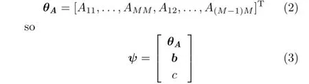
Before defining more notation we note that A can be assumed to be symmetric，without loss ofgenerality，as explained in Appendix A.Positive definiteness is determined from the eigenvalues. Letting ψ denote each element of A，b，and c.Further，let θAdenote the values in ψ that correspond to the values in A，i.e.，

The data from the input point cloud are collected into a data matrix X= ［x0，...，x‘，...，xN］T，so that

where x is an arbitrary column of X，and

In order to use Bayesian statistics，an additive noise model is assumed on each of the data points，i.e.，we assume that

where ε～ N（0，I）is a single draw from a unit multivariate Gaussian distribution.

In order to solve the matrix equation Xψ=0，without a prior on ψ one can find the eigenvector corresponding to the smallest eigenvalue of XTX.If we consider the following eigenvalue problem:

it is sufficient to find an eigenvector v associated with eigenvalue s=0.Existence of such a solution is guaranteed if the matrix XTX is singular.In practice，however，we take the smallest eigenvalue.

The solution to Eq.（7）is a least-squares solution of the equation||Xψ||2=0 since the value||Xψ||2is minimal when all of the partial derivatives with respect to ψ are zero.Consider

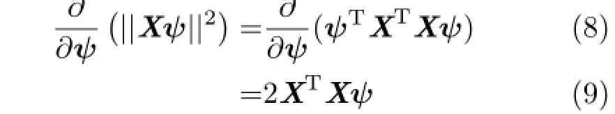
Setting Eq.（9）equal to zero and dividing out the constant，one can see that a minimal solution using eigenvalue decomposition is a least-squares estimate.

Theleast-squaresestimateintroducedabove places no constraint on the matrix A，and therefore can produce a matrix with negative eigenvalues.If one wishes to ensure that the matrix is an ellipsoid，for example，A is required to have a full set of positive eigenvalues.This is what motivates our use of Bayesian statistics.Not only does the noise model explicitly consider Gaussian errors，but it also allows us to enforce prior knowledge on the parameters. We extend the least-squares solution by introducing the model in Eq.（6）and then use Bayes’Law，which allows us to combine the likelihood of the data p（X|ψ）with a prior p（ψ）in order to produce the posterior:

The distribution p（X）is constant with respect to the parameters ψ and so we replace it with the proportionality operator（∝）.This is useful because traditionally，one would compute p（X）=which can be intractable.Certain properties are maintained across proportionality，for example，the maximum of p（ψ|X）is the same as the maximum of κp（ψ|X）for any κ.Since we only seek a maximum a priori estimate of the parameters，we only use equivalence of distributions up to proportionality.

With a careful choice of prior（discussed in Section 4），one can find the maximum a priori estimate of the parameters，given the data，by finding zeros of the log-posterior derivatives.In the context of fitting a general quadric and following from Eq.（6），we assume additive Gaussian noise on Eq.（1）in which case the likelihood is taken to be

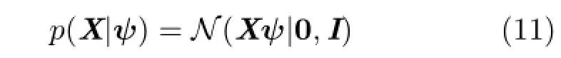
In other words，the errors in computing Eq.（1）are jointly Gaussian，with a spherical unit covariance I.Theassumptionofasphericalcovariance isequivalenttosayingthatthevariablesare independent，given the parameters ψ.This is true，since the error from the original surface of one point tells us nothing about the error of a neighbouring point.The covariances are assumed to be identical as a matter of simplicity.The identity is chosen rather than some scalar multiple，since the parameter becomes superfluous when the prior is introduced. The hyper-parameter σ（introduced later in the text）provides all of the information necessary to model the surface.

It would be possible at this point to use a prior for the vector ψ.Rather than doing this we introduce a bijection between A and ψ through the vector θ defined in Section 3.This allows the hyper-parameters to be set in terms of the matrix rather than the somewhat unintuitive values of ψ.In fact，using a matrix normal on A with scalar parameters is equivalent to assuming a multivariate Gaussian on the first elements of ψ.

We only place a prior distribution over the matrix A since it contains information about the shape of the surface.This is discussed in detail in Section 7，with the choice of hyper-parameters discussed more in Section 4.

The matrix normal distribution is defined as

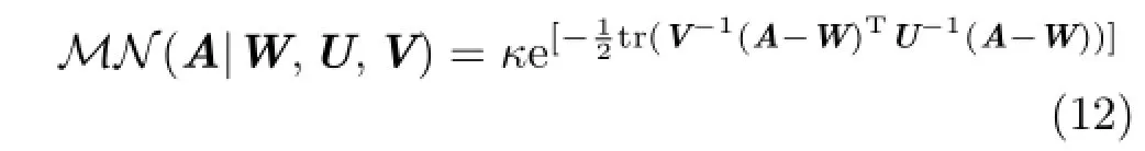
where W，U，V∈RM×Mand

The posterior is then found by multiplying Eq.（11）by Eq.（12）to give

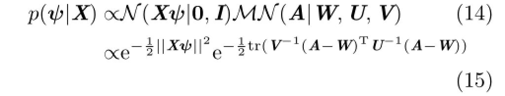
If we then choose U=V=σI，and ensure that W is diagonal and symmetric，the posterior can be simplified to

Taking the natural log and then the first partial derivative yields:

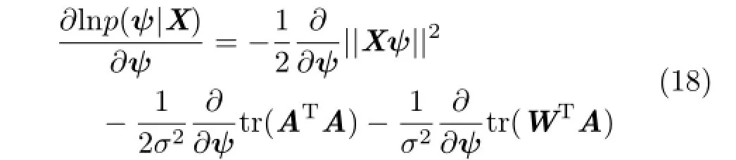
Before computing the vector derivatives，we first note the matrix derivatives for a symmetric A and W can be written as（see Ref.［25］for more details）:

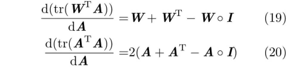
The operator◦is the Hadamard product for matrices，and produces a matrix of equal size by element wise multiplication:if S=Q◦R then Sij=QijRijfor each i and j.More intuitively，Eqs.（19）and（20）represent a doubling of all the offdiagonal elements，leaving the diagonals unchanged. Since A is symmetric we change notation for the derivatives and set

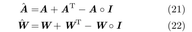
The final derivative can then be calculated as

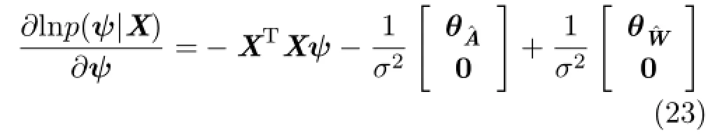
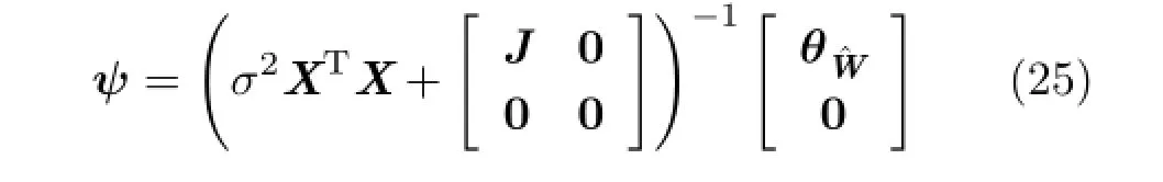
In the final step we separate ψ from X and σ by distributing multiplication over addition.Here ψ depends on A and θˆAonˆA.Let the matrix J be a diagonal matrix which takes a value of 1 on the diagonal when the corresponding value of θˆAis a diagonal element，and 2 otherwise.Setting the partials to zero it then follows that

Rearranging yields

4　Choice of prior

We use a matrix normal prior rather than a Wishart or inverse Wishart prior for the matrix A.The Wishart distributions are commonly used，well principled，and suitable for use with empirical data. However，computing a maximum a priori estimate in a similar fashion to that used in the previous section leads to a solution that must be determined by search，as opposed to the closed-form of Eq.（25）. The requirement that Wishart and inverse Wishart matrices are symmetric positive definite is another limitation，particularly if cylinders or hyperboloids are necessary.Section 7 discusses how to construct a mean matrix W in order to favour different shapes of surface.

The prior is only cast over the matrix A since the parameters b and c contain information about the center and also the width of the resulting surface.These values are also coupled，in the sense that a change in center affects both b and c. Section 6 discusses how to extract the center and width from the parameters，but their relationship is pathological.Constraining A alone provides just enough information on the shape of the surfaceto ensure that it does not become a hyperboloid，without affecting the quality of the fit.

The matrices U and V determine the variance of the matrix A from the mean W.Smaller values more strongly favour the mean as opposed to the data.For our experiments we simply choose the parameter σ∈R+，which gives control over how close the matrix A is to the identity.The value σ is free，in the sense that it can be chosen arbitrarily or depending on a larger dataset.The results in Section 8 describe how it is chosen for our experiments；however，it could also be computed using a training set containing prior information about the variance of the observed quadric from the mean.

5　3D data

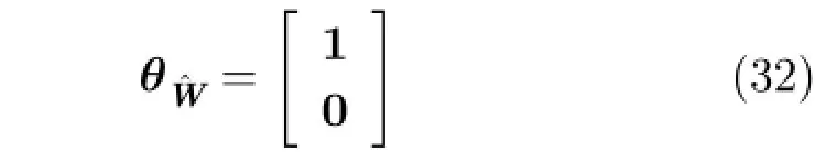
The results in Section 3 apply to data of arbitrary dimension.This section provides explicit formulae for 3 dimensions.We note that the same principles apply for 2 dimensional data，allowing us to model ellipses and hyperbola.

The parameters A and b can be written as follows:

In this case ψ is defined as

The matrix X is the quadratic data matrix:

The matrix J is then taken to be

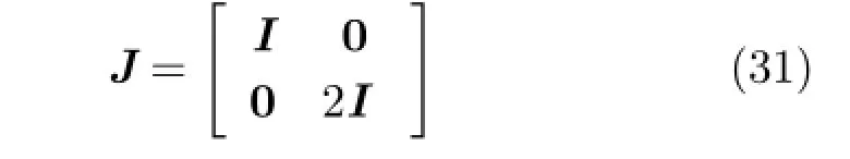
and

6　Parametrisation

The quadric can be parameterised by finding the transformation between the canonical shape，such as the unit sphere，and the resulting surface.

Consider the following:

Multiplying out and rearranging leads to

If we then take

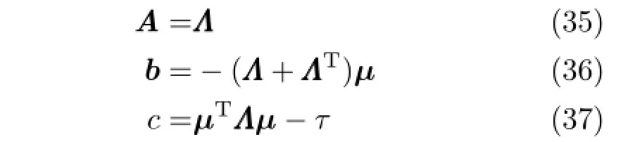
it can be seen that Eq.（1）takes on a canonical form of yTWy=1 after an affine transformation of the data，where W is a diagonal matrix with entries from the set｛1，0，-1｝.

For an ellipsoid，the matrix W is the identity. Faces and vertices on a unit sphere are generated usingasphericalcoordinatesystem，andwe transform only the vertices.Letting v be an arbitrary vertex on the unit sphere，and USUT=A be the eigendecomposition of A （A is Hermitian，so UT=U-1），it follows that

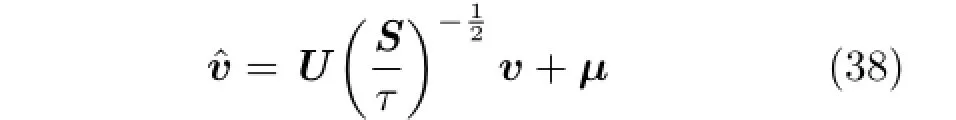
whereˆv is the required ellipsoid vertex.The same principle can be used for any canonical shape，including cylinders，ensuring that the principal axis is aligned with the zero entry of W.

Alternative methods exist for computing the solutions of Eq.（1）:isosurface algorithms，for example.A parametric approach is beneficial for its speed；however，it then also requires algebraic methods for merging with other surfaces，which can become complicated.

7　Eigendecomposition

The shape of the quadric can be determined by analysing the eigenvalues of A.

Since A is real and symmetric it is a special case of a Hermitian matrix，and so it follows that all of its eigenvalues are real.In the case of a symmetric positive definite matrix all of the eigenvalues are positive，and so the quadric forms an ellipsoid.If any of the eigenvalues are zero then the axis of the corresponding eigenvector is indeterminate；in the case of 2 positive eigenvalues it is a cylinder，for example.A single negative eigenvalue leads to a hyperboloid.

Thefinalclassificationscanbeobtainedby studyingthecanonicalformofthequadricintroduced in Section 6，yTWy=1，where y is an affine transformation of the arbitrary data values z，and W is a diagonal matrix.Multiplying this equation out for different combinations of sign on the diagonal of W reduces to a scalar equation which can be compared to studied quadratic forms，as presented in Andrews and S´equin［3］.

It is important to note that Eq.（1）is not only invariant to scale，but also negation，in the sense that multiplying the whole equation by a scalar α∈R does not change the solution set.Consider the following expansion:

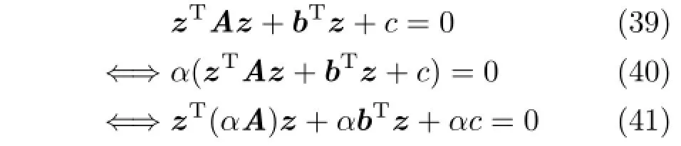
Further，let A=USUTbe the eigendecomposition of A.Then αA=UT（αS）U.This means that a scaling and negation of the eigenvalues of A only affects the other parameters，but not the solutions，e.g.，a full set of negative eigenvalues yields the same solution as a full set of positive eigenvalues.Since the signs of the eigenvalues of A are the same as the signs of the diagonal entries of W we can relate them to the shape of the surface.

A range of different surface shapes is attainable in this way.For example，a hyperboloid can be made from two negative and one positive eigenvalues，which is the same as two positive and one negative eigenvalues.A table showing the classification of the surface for different eigenvalues is shown in Table 1，and represents only a sample of the possible combinations.We note that the parameters b and c also have an affect on the shape.For example，if b=0 and we have one positive eigenvalue and two zero，the resulting shape is no longer a paraboloid but a pair of planes.Examples of these shapes can be seen in Fig.1.

8　Results

The results consider two scenarios.Firstly，it is shown that the method is able to perform well on data drawn from simulated quadrics，ellipsoids with known parameters.The algorithm is then shown to perform well on empirical data from a collection of 3D point clouds.The results are compare to quadric fitting without a prior and also against the work of Li and Griffiths［12］，who solve a generalised eigenvalue problem similar to that of Ref.［11］.

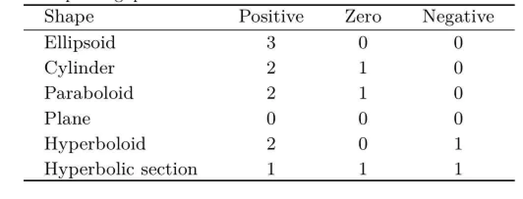
Table 1　Relationship between eigenvalues and shape of the corresponding quadric

The work presented by Li and Griffiths is a candidate example of a modern ellipsoid fitting algorithm，from the larger set of algorithms available （e.g.，Refs.［2-8］）.Our method is a Bayesian model，which allows us to provide a parameter which expresses a measure of how close the shape should be to a canonical shape，such as a sphere.Rather than comparing to all other algorithms we simply show that a hard constraint to fit an ellipse does not always lead to the best fit to the data，particularly when there is a large percentage of missing or excess noise.

In the final section of the results，we give an example of a fit to a simulated hyperboloid，primarily to show that our algorithm also works for different surface types.It also demonstrates the value in choosing different diagonals on the mean matrix W.

8.1Algorithmic complexity

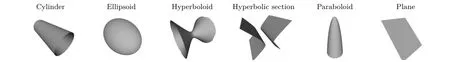
Fig.1　A collection of canonical quadric shapes.

One of the most attractive attributes of a direct method for fitting，such as ours and Refs.［12］or［11］，is its efficiency.A well known alternative is to compute the squared Euclidean（or geometric）distance between each point and the surface，and then minimise the sum of squares［9］.This isdifficult since computing the Euclidean distance is a non-linear problem （see Refs.［26，27］for more details），and the complexity is dependent on a polynomial root finding algorithm.Minimising the sum of squared errors in this way requires a nonlinear least-squares algorithm such as Levenberg-Marquardt.Computing the error alone has an order of O（NM3），which is a lower bound on the final fitting algorithm as it involves iteratively computing the error and parameter gradients at each step.It is possible，however，to approximate the distance function，as shown in Refs.［1］and［6］，and fit using generalised eigenvalues or using a linear leastsquares estimate；these methods have a much lower complexity，but do not allow us to use a Bayesian prior when fitting.

The complexity of the algorithm presented in the paper arises in the computation of the scatter matrix XTX in Eq.（25），which is O（NM2）；the subsequent matrix operations have much lower complexity（O（M3）at worst）.This makes ours an efficient approach，particularly since the scatter can be computed independently of the value σ. Faster algorithms exist for computing covariances，for example Ref.［28］，at the expense of memory，althoughitmaybegenerallyquickertouse parallel computation，such as a GPU，to improve performance.

8.2Simulated data

We first show results on a simulated dataset.Data is drawn from an ellipsoid of known dimensions，some of the data is removed，and spherical Gaussian noise is added.We show that with the correct choice of hyper-parameters，the Bayesian method fits best.

Figure 2 provides an example of fitting an ellipsoid to a simulated dataset，with missing data.In this experiment we only use 30%of the training data from the original ellipsoid and add Gaussian noise with a standard deviation of 0.01.It can be seen from the results that a value of σ=10 produces a result most plausibly in agreement with the original，whereas the result of fitting with no prior produces a hyperboloid. It is

clear from this example that lower values of σ produce a result closer to a sphere.

In order to determine the quality of the fit，we compare the vertices on the original quadric with the fitted quadric using the Hausdorff distance.Firstly，the distance between a point xi∈X and a point cloud Y=｛y0，...，yN｝is taken to be

The Hausdorff distance is then:

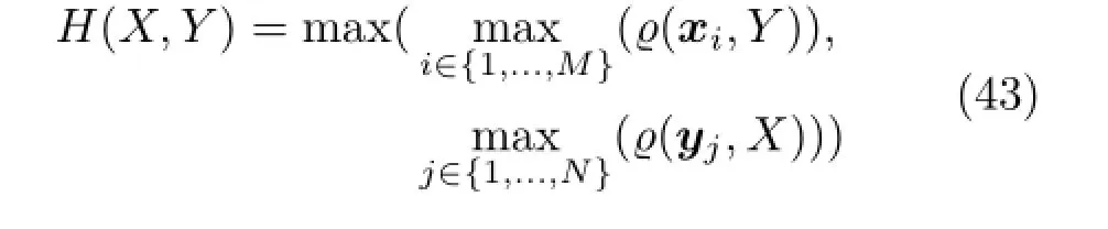
Fig.2　A collection of ellipses fitted to data.Bottom:results of fitting with a prior.Top:results of fitting with no prior.The first two images are the point cloud and the ellipsoid that they were generated from.

The first experiment considers how each of the algorithms perform when there is missing data.We generate an arbitrary ellipsoid and remove N%of the data，and add spherical Gaussian noise with 0.01 standard deviations.The parameters of the ellipsoid are drawn as follows:

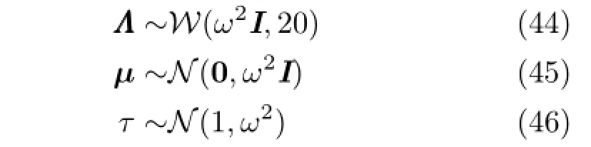
with ω2=0.01.The parameters A，b，and c are computed as in Section 6.The percentage of data removed is varied between 10%and 100%，and we choose the hyper-parameter 0.1＜σ＜30 which produces the best Hausdorff distance.Using a multivariate matrix normal prior is compared with （1）using no prior at all and（2）the ellipsoid specific least-squares method of Li and Griffiths［12］.

The results of the first experiment can be seen in Fig.3.Our method consistently outperforms both methods，although the distance drops below the standard deviation in Gaussian noise in all methods after 60%of the data is used.Fitting without a prior also gives reasonable results if enough of the data is used.

Inthesecondsimulationexperimentwe demonstrate how the method is robust to noise by varying the amount of additive Gaussian noise added to each sampled ellipsoid.We denote the noise level byˆτ.In order to demonstrate the quality of fit over a range of values we sample 10 quadrics and compute error statistics.In this experiment we use 100%of the points，i.e.，there is no missing data. The hyper-parameter is fixed at σ=10.

The results from the second experiment can be seen in Fig.4.Our method produces a Hausdorff distance which is comparable to Ref.［12］for lower values ofˆτ，while asˆτ increases the use of a prior proves to be beneficial.Although fitting without a prior gives reasonable results whenˆτ is small，it becomes very inaccurate whenˆτ is greater than 0.06. This tends to be due to negative eigenvalues in the matrix A which does not produce an ellipsoid.

In order to show that the algorithm works for other types of quadric surface，we simulated a hyperboloid and removed a percentage of the points.Three quadrics were fitted to the data using different priors for each of:an ellipsoid，no prior，and a hyperboloid.For the ellipsoid，W=I and σ= 1e-6；for the hyperboloid W=Diag（-1，1，1）and σ=10.Note that the variance for the ellipsoid needs to be low enough or it will favor a different shape.The hyperboloid hyper-parameter is aligned with the x-axis，as for the simulated data，based on our knowledge of the shape.Fitting without a prior chooses the hyperboloid’s medial axis to be aligned with the z-axis.The results of this experiment can be seen in Fig.5.The original quadric is in the top left of the figure.It is clear that using a hyperboloid prior is the best option for this data.

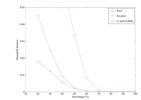
Fig.3　The Hausdorff distance for a varying amount of missing data.

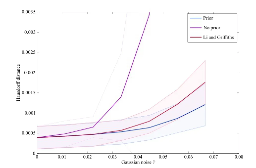
Fig.4　The Hausdorff distance for a varying amount of Gaussian noise.The shaded regions represent one standard deviation from the mean.

8.3Empirical data

We provide some examples which demonstrate the use of our algorithm on real data from point clouds extracted from a visual structure from a motion pipeline.In this scenario，regions of the point cloudcan be left without any reconstructed points.An example is shown in Fig.6.A smooth surface must be fitted to the roof of the phone box，presenting a challenge for most surface fitting algorithms due to the noisy and shapeless extracted points.Previous algorithms either do not fit at all，such as the one in Li and Griffiths［12］，or do not allow control over the curvature of the data，which is the case when using no prior.The surface gradient can be chosen to match the roof curvature by varying σ and produces a final result as shown.

Some examples of the algorithm on point cloud dataareshowninFig.7.Thepointclouds are computed from a collection of photographs comprising a post box，rugby ball，and roof.The surfaces are visually plausible even when there are large regions of missing data.This is particularly visible on the roof data，for which only the front is visible in each of the photographs.

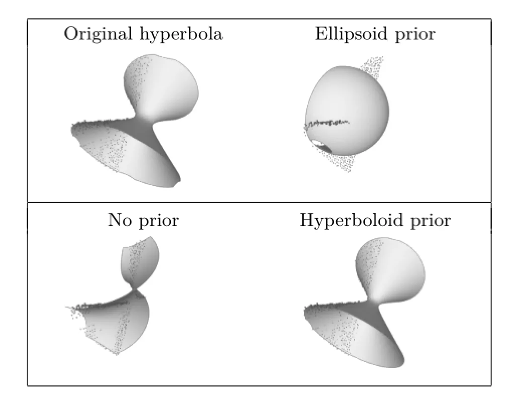
Fig.5　Fitting a hyperbola using a variety of different priors.The original points are shown as black dots.

9　Conclusions

We conclude by observing that state of the art methods for quadric fitting give reasonable results on noisy point clouds.Our algorithm provides a means to enforce a prior，allowing the algorithm to better fit the quadric that the points were drawn from，particularly when there is missing data or a large amount of noise.This has a practical use for real datasets，since it allows a user to specify the curvature of the surface where there are few points available.

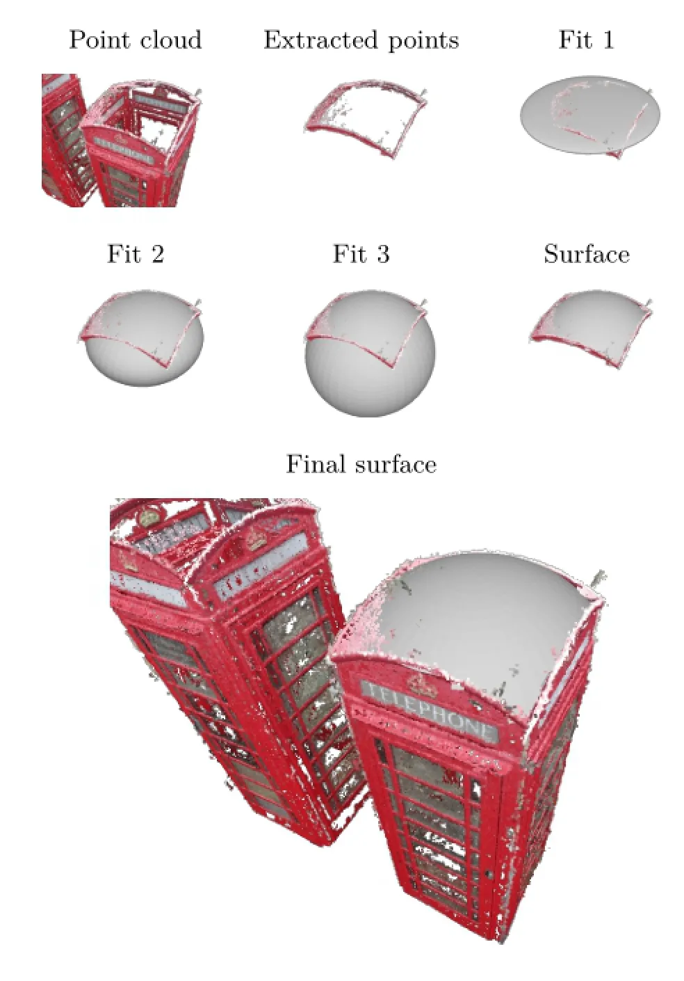
Fig.6　Phone box dataset.The top left shows the original point cloud and the extracted points that a quadric must be fitted to，followed by 3 examples with varying sigma values and the final surface at the bottom right.

Appendix A　Symmetry of the matrix A

The matrix A is assumed symmetric without loss of generality.This is possible since the function:

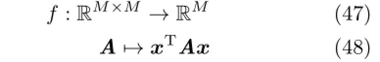
is not injective for any x∈RM.For example，if we take

which is a symmetric matrix，then

Since xTATx is a scalar，it is also symmetric，and soIt then follows that

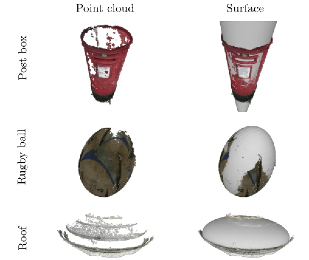
Fig.7　Some examples of the quadric fitting algorithm on point cloud data.

The choice of symmetry then follows，because if A，b，and c satisfy xTAx+bTx+c=0，then so does B，and B is symmetric.

References

［1］Taubin，G.Estimation of planar curves，surfaces，andnonplanarspacecurvesdefinedbyimplicit equations with applications to edge and range image segmentation.IEEE Transactions on Pattern Analysis and Machine Intelligence Vol.13，No.11，1115-1138，1991.

［2］Ahn，S.J.；Rauh，W.；Cho，H.S.；Warnecke，H.-J.Orthogonal distance fitting of implicit curves and surfaces.IEEE Transactions on Pattern Analysis and Machine Intelligence Vol.24，No.5，620-638，2002.

［3］Andrews，J.；S´equin，C.H.Type-constrained direct fitting of quadric surfaces.Computer-Aided Design and Applications Vol.11，No.1，107-119，2014.

［4］Atieg，A.；Watson，G.A.A class of methods for fitting a curve or surface to data by minimizing the sum of squares of orthogonal distances.Journal of Computational and Applied Mathematics Vol.158，No. 2，277-296，2003.

［5］Gander，W.；Golub，G.H.；Strebel，R.Leastsquares fitting of circles and ellipses.BIT Numerical Mathematics Vol.34，No.4，558-578，1994.

［6］Luk´acs，G.；Martin，R.；Marshall，D.Faithful leastsquares fitting of spheres，cylinders，cones and tori for reliable segmentation.In:Lecture Notes in Computer Science，Vol.1406.Burkhardt，H.；Neumann，B.Eds. Springer Berlin Heidelberg，671-686，1998.

［7］Petitjean，S.A survey of methods for recovering quadrics in triangle meshes.ACM Computing Surveys （CSUR）Vol.34，No.2，211-262，2002.

［8］Ruiz，O.；Arroyave，S.；Acosta，D.Fitting of analytic surfaces to noisy point clouds.American Journal of Computational Mathematics Vol.3，No.1A，18-26，2013.

［9］Rouhani，M.；Sappa，A.D.Implicit polynomial representation through a fast fitting error estimation. IEEE Transactions on Image Processing Vol.21，No. 4，2089-2098，2012.

［10］Pratt，V.Direct least-squares fitting of algebraic surfaces.ACM SIGGRAPH Computer Graphics Vol. 21，No.4，145-152，1987.

［11］Fitzgibbon，A.；Pilu，M.；Fisher，R.B.Direct least square fitting of ellipses.IEEE Transactions on Pattern Analysis and Machine Intelligence Vol.21，No. 5，476-480，1999.

［12］Li，Q.；Griffiths，J.G.Least squares ellipsoid specific fitting.In:Proceedings of Geometric Modeling and Processing，335-340，2004.

［13］Halir，R.；Flusser，J.Numerically stable direct least squares fitting of ellipses.In:Proceedings of the 6th International Conference in Central Europe on Computer Graphics and Visualization，Vol.98，125-132，1998.

［14］Dai，M.；Newman，T.S.；Cao，C.Least-squares-based fitting of paraboloids.Pattern Recognition Vol.40，No. 2，504-515，2007.

［15］Subrahmonia，J.；Cooper，D.B.；Keren，D.Practical reliable Bayesian recognition of 2D and 3D objects using implicit polynomials and algebraic invariants. IEEE Transactions on Pattern Analysis and Machine Intelligence Vol.18，No.5，505-519，1996.

［16］Cohen-Steiner，D.；Alliez，P.；Desbrun，M.Variational shape approximation.ACM Transactions on Graphics Vol.23，No.3，905-914，2004.

［17］Wu，J.；Kobbelt，L.Structure recovery via hybrid variational surface approximation.Computer Graphics Forum Vol.24，No.3，277-284，2005.

［18］Yan，D.-M.；Liu，Y.；Wang，W.Quadric surface extraction by variational shape approximation.In: Lecture Notes in Computer Science，Vol.4077.Kim，M.-S.；Shimada，K.Eds.Springer Berlin Heidelberg，73-86，2006.

［19］Schnabel，R.；Wahl，R.；Klein，R.Efficient RANSAC for point-cloud shape detection.Computer Graphics Forum Vol.26，No.2，214-226，2007.

［20］Li，Y.；Wu，X.；Chrysathou，Y.；Sharf，A.；Cohen-Or，D.；Mitra，N.J.GlobFit:Consistently fitting primitives by discovering global relations.ACM Transactions on Graphics Vol.30，No.4，Article No. 52，2011.

［21］Ohtake，Y.；Belyaev，A.；Alexa，M.；Turk，G.；Seidel，H.-P.Multi-level partition of unity implicits. In:Proceedings of ACM SIGGRAPH 2005 Courses，Article No.173，2005.

［22］Hamann，B.Curvature approximation for triangulated surfaces.In:Computing Supplementum，Vol.8.Farin，G.；Noltemeier，H.；Hagen，H.；Kndel，W.Eds. Springer Vienna，139-153，1993.

［23］Vona，M.；Kanoulas，D.Curved surface contact patches with quantified uncertainty.In:Proceedings of IEEE/RSJ International Conference on Intelligent Robots and Systems，1439-1446，2011.

［24］Powell，M.W.；Bowyer，K.W.；Jiang，X.；Bunke，H.Comparing curved-surface range image segmenters. In:Proceedings of the 6th International Conference on Computer Vision，286-291，1998.

［25］Petersen，K.B.；Pedersen，M.S.The Matrix Cookbook. Technical University of Denmark.Version:November 15，2012.Available at https://www.math.uwaterloo. ca/vhwolkowi/matrixcookbook.pdf.

［26］Lott，G.K.Direct orthogonal distance to quadratic surfaces in 3D.IEEE Transactions on Pattern Analysis and Machine Intelligence Vol.36，No.9，1888-1892，2014.

［27］Eberly，D.Distance from a point to an ellipse，an ellipsoid，or a hyperellipsoid.Geometric Tools，LLC，2011.Available at http://www.geometrictools.com/ Documentation/DistancePointEllipseEllipsoid.pdf.

［28］Kwatra，V.；Han，M.Fast covariance computation and dimensionality reduction for sub-window features in images.In:Lecture Notes in Computer Science，Vol. 6312.Daniilidis，K.；Maragos，P.；Paragios，N.Eds. Springer Berlin Heidelberg，156-169，2010.

DanielBealeisapost-doctoral research officer at the University of Bath.He obtained his Ph.D.degree in computer science and master degree of mathematics（M.Math.）from the University of Bath.He has worked in industrial positions as a software and systems engineer.His interests are in the application of mathematics，statistics，and probability theory to problems in computing，particularly in the area of computer vision.

Yong-LiangYangisalecturer （assistant professor）in the Department of Computer Science at the University of Bath.He received his Ph.D.degree and master degree in computer science from Tsinghua University.His research interests include geometric modelling，computational design，and computer graphics in general.

NeillCampbellisalecturerin computer vision，graphics，and machine learning in the Department of Computer ScienceattheUniversityofBath. Previously he was a research associate at University College London（where he is an honorary lecturer）working with Jan Kautz and Simon Prince.He completed his M.Eng.and Ph.D.degrees in the Department of Engineering at the University of Cambridge under the supervision of Roberto Cipolla with George Vogiatzis and Carlos Hern`andez at Toshiba Research.His main area of interest is learning models of shape and appearance in 2D and 3D.

DarrenCosker is a Royal Society Industrial Research Fellow at Double Negative Visual Effects，London，and a reader（associate professor）at the University of Bath.He is the director oftheCentrefortheAnalysisof Motion，Entertainment Research and Applications（CAMERA），starting from September 2015.Previously，he held a Royal Academy of Engineering Research Fellowship，also at the University of Bath.His interests are in the convergence of computer vision，graphics，and psychology，with applications in movies and video games.

PeterHall is a professor of visual computing at the University of Bath. His research interests focus around the use of computer vision for computer graphicsapplications.Heisknown forautomaticallyprocessingreal photographsandvideointoart，especiallyabstractstylessuchas Cubism，Futurism，etc.More recently he has published papers on classification and detection of objects regardless of how they are depicted such as photos，drawings，paintings，etc.He is also interested in using computer vision methods to acquire 3D dynamic models of complex natural phenomena such as trees，water，and fire for use in computer games，TV broadcast，and film special effects.

Open AccessThe articles published in this journal aredistributedunderthetermsoftheCreative Commons Attribution 4.0 International License（http:// creativecommons.org/licenses/by/4.0/）， whichpermits unrestricted use，distribution，and reproduction in any medium，provided you give appropriate credit to the original author（s）and the source，provide a link to the Creative Commons license，and indicate if changes were made.

Other papers from this open access journal are available free of charge from http://www.springer.com/journal/41095. To submit a manuscript，please go to https://www. editorialmanager.com/cvmj.