On a Dual Risk Model Perturbed by Diffusion with Dividend Threshold∗

Hui ZHI Jiangyan PU

1 Introduction

The optimal dividend problem proposed by de Finetti[10]in the XVth international congress of actuaries is to find the dividend-payment strategy that maximizes the expected discounted value of dividends which are paid to the shareholders until the company is ruined or bankrupt.He assumed that the annual gains of a stock company are independent and identically distributed random variables that only take the value−1 or+1.He also claimed that the optimal dividend strategy is a barrier strategy,that is,any surplus above a certain level should be paid to the shareholders immediately as dividends.

The optimal dividend problem in the classical compound Poisson model was first discussed by B¨uhlmann[8].[2,16]studied the problem with a bounded dividend rate in a Brownian motion model.They assumed that only dividend strategies with a ceiling for the dividend rate are admissible.They showed that the optimal dividend strategy is then a threshold strategy,that is,dividends should be paid to the shareholders at the maximal admissible rate once the surplus exceeds a certain threshold.A down-to-earth calculation can be found in Gerber and Shiu[14].

In insurance mathematics,the classical risk model has drawn the attention from researchers for decades.The surplus in the classical model at time t can be presented as

where u is the initial surplus,c is the premium rate,and S(t)usually modeled by a compound Poisson process are the aggregate claims by time t.In this model,the optimal dividend strategy is not a barrier strategy in general(see[8]).In recent years,quite a few papers discussed the dual model to the classical insurance model.In the dual model,the surplus at time t is

For example,Avanzi et al.[4]studied the expected total discounted dividends until ruin under the barrier strategy.Avanzi and Gerber[5]studied a dual model perturbed by diffusion and discussed how to determine the optimal value of the barrier.Ng[19]studied the optimal dividend problem under the bounded dividend rate constraint and calculated the optimal threshold by means of integro-differential equations.

In this paper,we discuss the dual risk model perturbed by diffusion with a bounded dividend rate constraint.Now the surplus at time t is

We assume E(S(1))−c＞0,which means the expected gain per unit time is positive.The diffusion term adds uncertainty to the expenses.It makes the model closer to the reality.Indeed,the expense rate can not be a constant in finance.Such a bounded dividend rate constraint makes our optimal strategy turn out to be a threshold strategy,that is,the company pays dividends at an admissible maximal rate when the surplus exceeds a threshold b.Comparing with the barrier strategy at the same level b,the time of ruin under the threshold strategy is longer,which makes the company prefer the threshold strategy.Indeed,the company with the barrier dividend policy will eventually go bankrupt,which is discrepant to the real cash fl ow.

This paper is inspired by[5,19].We formulate the problem and prove that the optimal strategy in our problem is a threshold strategy in Sections 2–3.In Section 4,we show that the expected total discounted dividends until ruin,denoted as V(u;b),can be characterized as the solution of a set of two second order integro-differential equations in conjunction with three boundary conditions.It is shown that V(u;b)can purely depend on the integro-differential equation finished by 0≤u≤b.We study the special cases where the pro fi ts distribution is an exponential or mixtures of exponential distributions.Section 5 introduces an alternative approach–the method of the Laplace transform–to obtain the expected total discounted dividends until ruin.Finally,we introduce the optimal threshold b∗in Section 6.With the help ofand Vu(b∗;b∗)=1,b∗and V(u;b∗)can be determined by the method of the Laplace transform.

2 Problem Formulation

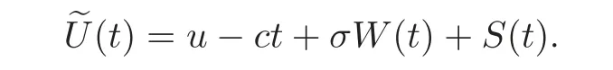
We consider the dual risk model perturbed by diffusion.The surplus process{X(t)}is given by

Here u=X(0)is the initial surplus,and c is a positive constant which stands for the rate of expense.The aggregate pro fits process{S(t)}is assumed to be a compound Poisson process,i.e.,where{N(t)}is a Poisson process with a Poisson parameter λ and individual pro fit amount Yi’s are independent and identically distributed with the probability density function p(y),y≥0.{W(t)}is a standard Wiener process which is independent of{S(t)}and the volatility σ＞0 is a constant.The diffusion term adds uncertainty to the expenses which makes the model closer to the reality.

We now enrich the model.We assume that the dividends are paid to the shareholders according to some dividend strategies.Let D(t)denote the aggregate dividends paid from time 0 to time t,and then the modified surplus process at time t is

Let

be the time of ruin and

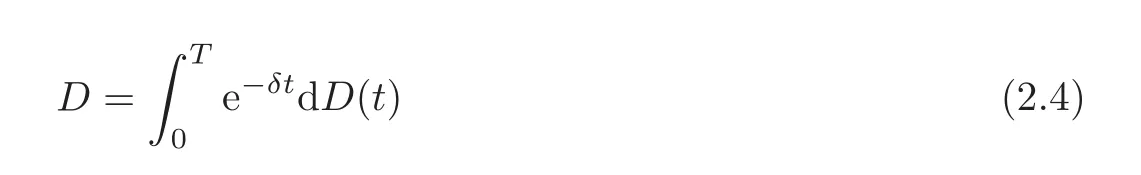
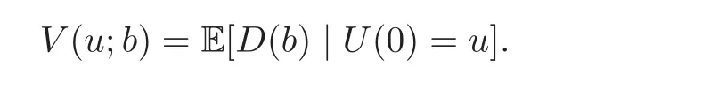
be the present value of all aggregate dividends until ruin,where δ＞ 0 is the force of interest to discount the dividends.The company looks for a dividend strategy to maximize the expectation of the random variable D.

For a given D(·),the cost functional is defined by

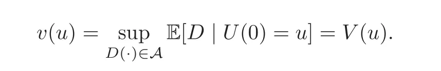
The value function is defined by

where A is a class of processes called admissible controls which will be described below.

We study this stochastic optimal control problem under the constraint that only dividend strategies with a dividend rate bounded by a ceiling are admissible.We call a dividend strategy admissible if it is non-negative,non-decreasing,absolutely continuous and rate bounded.Thus,we assume

where α ＜ ∞ is the dividend rate ceiling.

3 Dynamic Programming

3.1 HJB equation

Proposition 3.1 The value function V defined by(2.6)satisfies the Hamilton-Jacobi-Bellman(HJB for short)functional equation

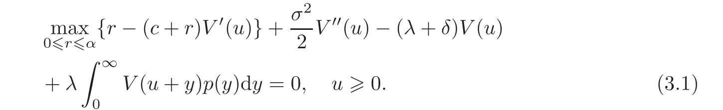
Proof We use Bellman’s dynamic programming principle to prove(3.1).We consider a small time interval[0,∈],∈＞ 0.Suppose that dividends are paid at rate r between time 0 and time∈,and then continue optimally.By conditioning on whether a jump occurs at the time interval[0,∈]and on the amount of the jump,we can obtain that the expectation of the present value of all dividends until ruin is

Since

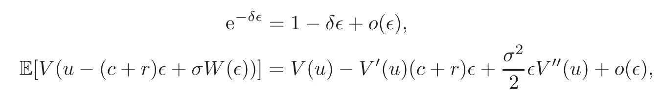
the expression(3.2)is equal to

Because V(u)is the optimal value,it must be equal to the maximum value of the expression(3.3),where r∈ [0,α].Thus,we obtain the functional equation(3.1).

On the left-hand side of the equation(3.1),the expression to be maximized is

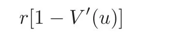
for r∈ [0,α].Thus,the optimal dividend rate at time 0 is

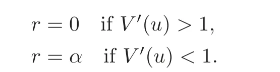
Then,at time t∈[0,T],the optimal dividend rate is

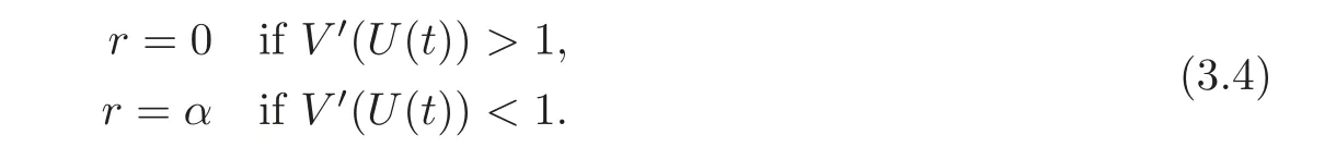
Such a dividend strategy has the character of a bang-bang strategy.

Remark 3.1(3.4)can be interpreted as follows:When V′(U(t))＞ 1,the company can be considered efficient,so it is best to leave all the funds with the company and pay no dividend.On the other hand,when V′(U(t))＜ 1,the company is inefficient,it is advantageous to pay out as many dividends as allowable.The problem of decision between dividend payout and plowback is a classical problem in corporate finance.

3.2 Verification of optimality

We have shown that the value function V satisfies the HJB equation(3.1).However,this does not guarantee that any solution of the HJB equation(3.1)is the value function.The following theorem(the verification theorem)shows that a strategy is indeed an optimal strategy if its corresponding cost functional satisfies the HJB equation(3.1).

Theorem 3.1 Suppose that v(u)satisfies the HJB equation(3.1).Then for all u≥0,suppose that v is a C2-function satisfying the HJB equation(3.1),and then,for all u≥0 and

D(·) ∈ A,we have that v(u) ≥ VD(u).Consequently,if there exists a D∗(·) ∈ A such that v(u)=VD∗(u),then

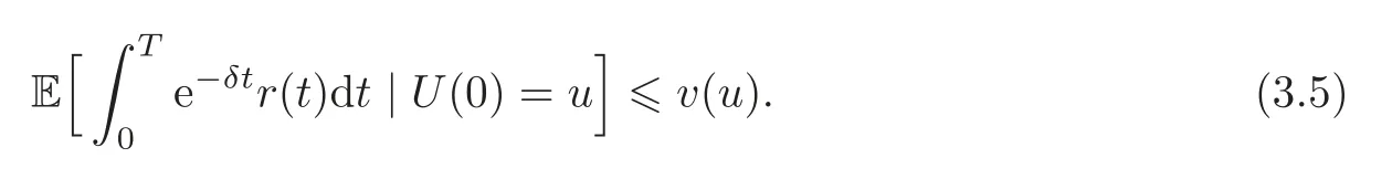
Proof Consider any admissible dividend strategies with dividend rate r(t)and surplus U(t)at time t.We claim that

To prove(3.5),we consider the compensated process

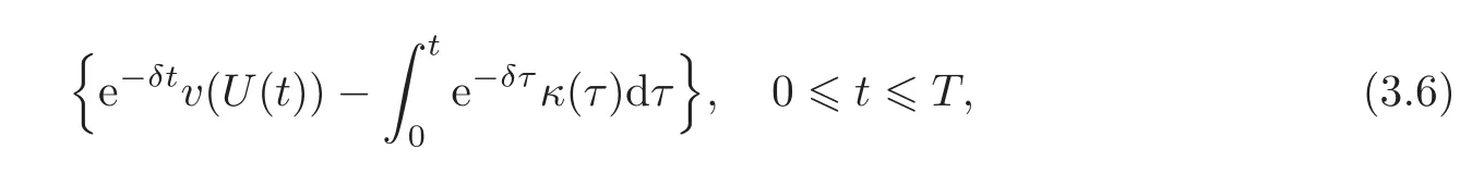
where

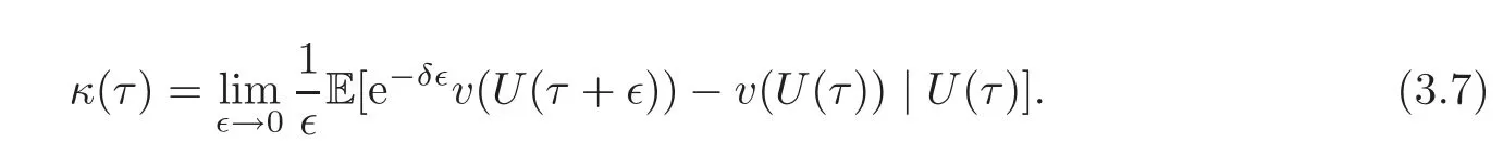
Note that κ(τ)is the generator of the Itdiffusion,and then(3.6)is a martingale(see[20,Theorem 7.3.3,p.123]).We have

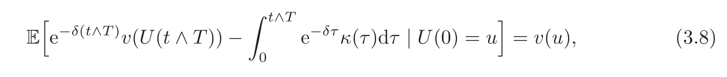
which implies

By a calculation similar to that by which we obtained(3.3),we see

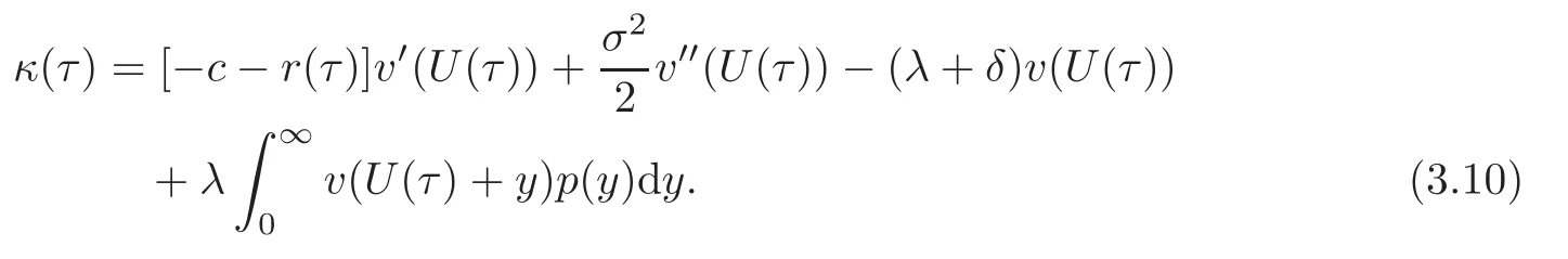
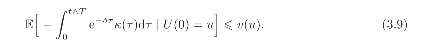
Because the function v(u)satisfies the HJB equation(3.1),the sum of r(τ)and the expression(3.10)can not be positive.That is,

Together with(3.9),we have

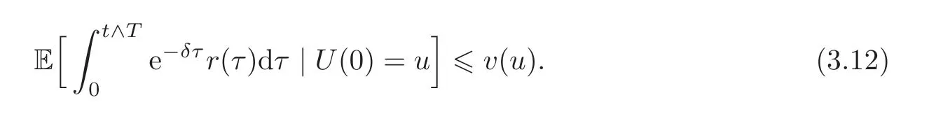
Finally,(3.5)can be obtained by taking the limit t→ ∞.Then we have v(u)≥VD(u).The remainder of the theorem is obvious,so the proof is completed.

4 Integro-Differential Equations

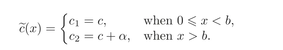
If the solution of the HJB equation(3.1)has the property that V′(x)＞ 1 for x ＜ b and V′(x)＜ 1 for x＞b,for some number b,then the optimal dividend strategy is particularly appealing:When 0＜U(t)＜b,no dividends are paid,otherwise,when U(t)＞b,dividends are paid at the maximal rate α.Such a dividend strategy is called a threshold strategy.After a threshold dividend strategy with a threshold level b applied,the dynamics of the surplus process U(t)become

where

The present value of all aggregate dividends until ruin is

where I is the identity operator.The expected present value of all aggregate dividends until ruin is

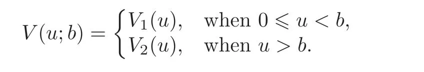
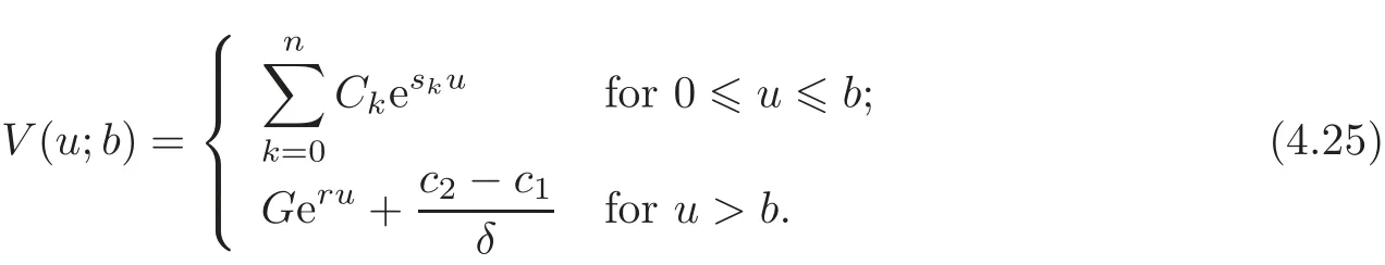
Since the surplus U(t)has different paths for 0 ≤ U(t)＜ b and U(t)＞ b,then we define

We derive a set of integro-differential equations finished by V(u;b)in the following proposition.

Proposition 4.1 The expectation of the discounted dividend V(u;b)satisfies the following integro-differential equations:When 0≤ u ＜ b,

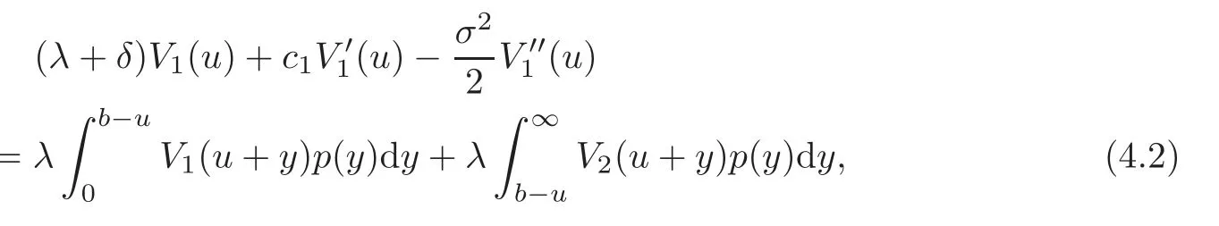
and when u＞b,

with the initial condition V1(0)=0,and continuity conditions

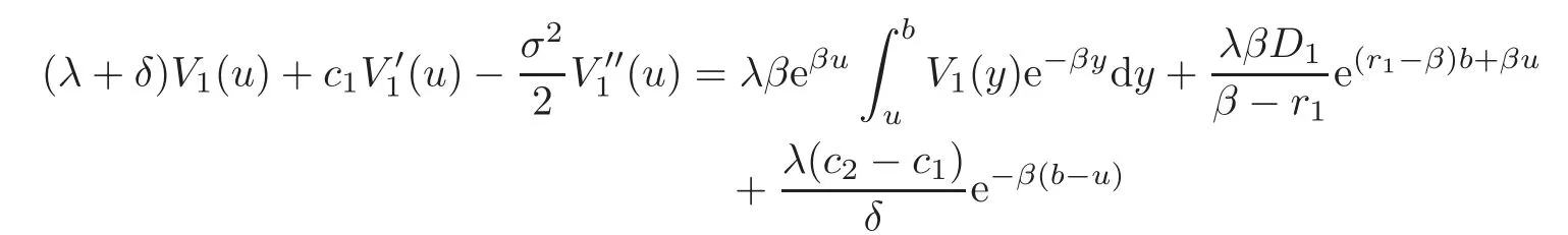
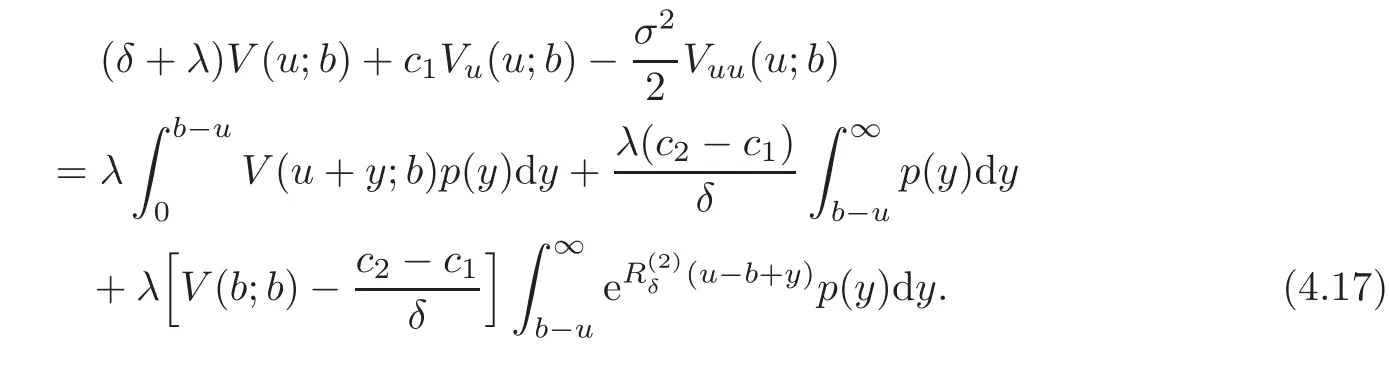
Proof Firstly,we consider the case where u ＞ b and fix a small enough time τ such that u −c2τ+σW(τ)＞ b.By conditioning on whether a jump occurs and on the amount of the jump at the time interval[0,τ],it follows that

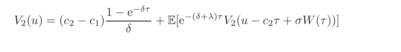
Combining with the identities

and

we subtract V2(u)on both sides of(4.4),divide by τ and let τ→ 0.This induces(4.3).

Using a similar argument,we can also derive the corresponding integro-differential equation finished by V1(u).

Since ruin occurs immediately if the initial surplus is zero and no dividend is paid,the initial condition holds.

Remark 4.1 Though V(u;b)and Vu(u;b)are continuous at b,it may not be the case for Vuu(u;b).Indeed,from(4.2),

while from(4.3),

As a result,

which implies that

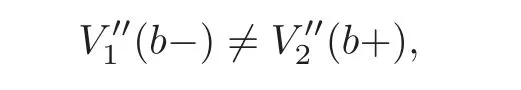
unlessThis fact will be used later in the determination of the optimal level of threshold.

Remark 4.2 For further reference,it is useful to rewrite the integro-differential equations as follows:When 0≤u≤b,

and when u＞b,

and for u＞b,

Remark 4.3 When σ=0,for 0≤u≤b,

These results were obtained in[19].

4.1 Explicit results for exponentially distributed pro fits

In this section,we obtain the explicit solution of(4.6)–(4.7)when jump amounts are exponentially distributed.

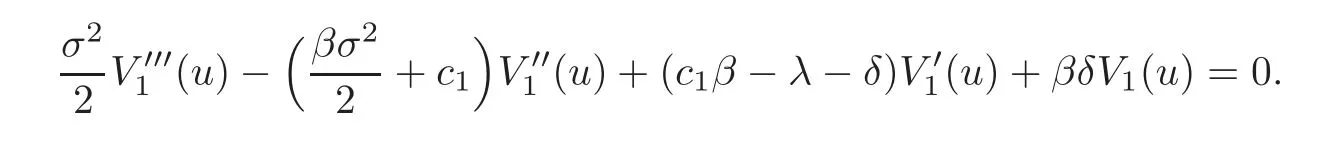
Let pro fits Yi’s follow an exponential distribution with p(y)= βe−βyfor y ＞ 0.Substituting the distribution density function into(4.7),we have,for u＞b,

Applying the operatorto both sides,we get

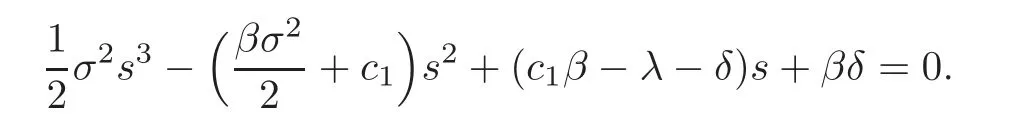
The third-order linear differential equation above has a particular solutionSince the characteristic equation of the differential equation

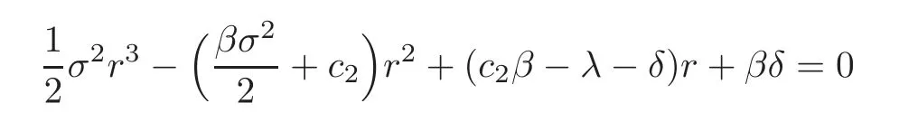
has a negative root r1and two positive roots r2,r3(r1＜0＜r2＜β＜r3),we obtain

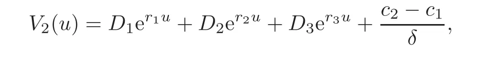
where D1,D2and D3are undetermined coefficients.From

it is clear that

We have D3≤0.To prove that D3=0,we consider the derivative of V2(u):

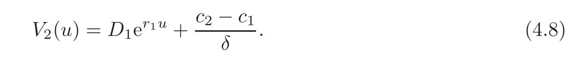
If D3＜0,then V′2(u)＜0 for sufficiently large values of u,which contradicts the fact that V2is increasing in u.Thus,D3=0 and D1＜0.Using exactly the same argument,we can also derive that D2=0.Therefore,

To solve V1,we substitute the expression for V2(u)above into(4.6)and obtain

for 0≤u≤b.Applying the operatorto both sides,we have

Hence

where E1,E2and E3are undetermined coefficients.s1,s2and s3(s1＜0＜s2＜β＜s3)are the solutions of the characteristic equation

Since V1(0)=0,we have

On the other hand,with the continuity condition:V1(b−)=V2(b+),we have

With the first-order continuity condition:we have

Substituting back the solution for V1(u)and V2(u)into(4.6),we have

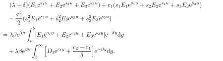
Since the expression above must be finished for all 0＜ u ＜ b,the sum of the coefficients of eβuis zero,i.e.,

We have(4.10)–(4.13)to solve for E1,E2,E3and D1.Then the solution for V(u;b)can be expressed as

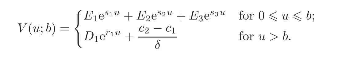
4.2 V(u;b)as a function of V1(u)

When pro fits follow an exponential distribution,we have

for D1＜0.In this section,we show that the presentation above holds for any other pro fit distribution,which implies that V(u;b)can be expressed as a function of V1(u).So it is not necessary to solve V2(u)explicitly.

Firstly,we need to deduce the generalized Lundberg fundamental equation,which plays an important role in the risk theory.

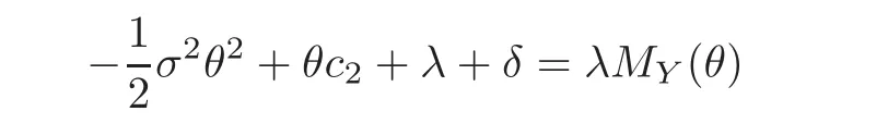
Lemma 4.1 Consider a compound Poisson jump-diffusion dual model,where no dividenddistribution policy is imposed and expenses are paid continuously at a constant rate c,

Then the Laplace transform of the time of ruin,φ(u),is given by

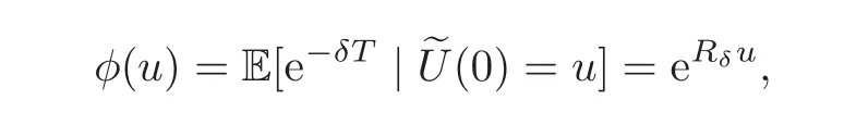
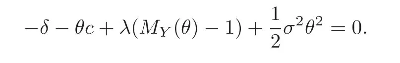
where Rδis the unique non-positive root of the generalized Lundberg fundamental equation

where MYis the moment-generating function of Yi.

Proof Consider a process{Zθ(t):t≥ 0}defined bySince{(t)}has independent and stationary increments,{Zθ(t)}is a martingale if and only if E(Zθ(t))=Zθ(0).This condition is equivalent to

Then,we obtain the generalized Lundberg fundamental equation

Let Rδbe the unique non-positive root of(4.14),and note that 0＜ ZRδ(t)≤ 1 for 0≤ t≤ T gives that{ZRδ(t∧ T)}is a bounded martingale.An application of the optional sampling theorem shows E(ZRδ(t∧ T))=ZRδ(0)for every t.By applying the dominated convergence theorem,we can obtain E(ZRδ(T))=ZRδ(0),which is the result asserted.

Remark 4.4 By considering the slope of λ(MY(θ)− 1)− θc+σ2θ2,it can be observed that Rδ=0 if and only if δ=0 and c ≥ λμ,where μ is the mean of Yi.Since we assume δ＞ 0,Rδwill be strictly less than 0 no matter the drift of{?U(t)}is positive or not.

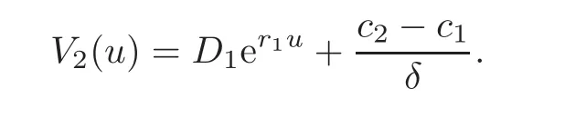
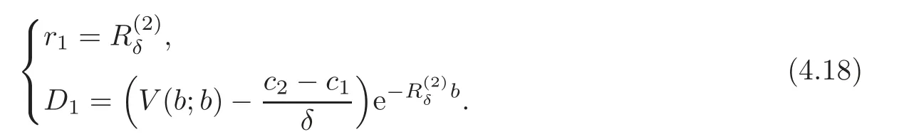
Theorem 4.1 For u＞b,

whereis the unique negative root of the generalized Lundberg fundamental equation

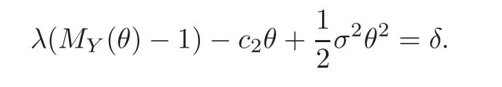
Proof Let χ =u−b and denote the first passage time until the surplus process descends χ units byWe consider a life status with the failure time.Dividends are paid at the rate(c2−c1)untilA life insurance of 1 payable at timediscounted at a continuously compounded rate of δ has the expected present valueaccording to Lemma 4.1.With the relation A+ δa=1,we haveSince the total discounted dividends until ruin are the sum of the continuous annuity payable untilwith a payment rate(c2−c1)and the discounted dividends until ruin after the first downcrossing level b,

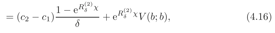
which is the result asserted.This method is discussed in[19].

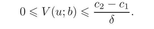
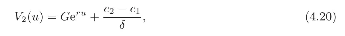
In view of Theorem 4.1,we do not need to solve V2(u)to obtain V(u;b)when 0≤u≤b.Instead,we can directly substitute(4.16)into(4.2)to obtain an integro-differential equation to solve V(u;b)when 0≤u≤b:

The equation above is analogous to Equation(2.4)in[5]with the exception of the term involving

Remark 4.5 When pro fi ts follow an exponential distribution,we have already proved

Together with(4.15),we can verify that

4.3 Mixtures of exponential distributions

In this section we show how V(u;b)can be calculated when

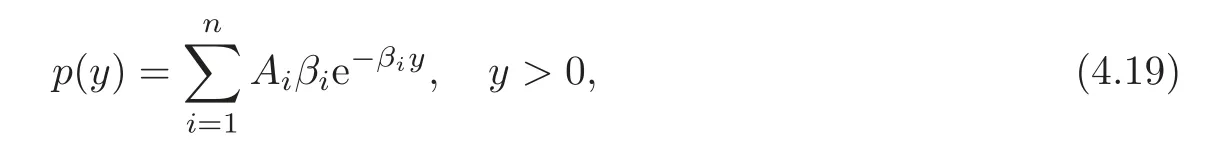
where β1＜ β2＜ β3＜ ···＜ βn,Ai＞ 0,and A1+A2+ ···+An=1.

For notational convenience,we write

where

The substitution of(4.19)in(4.6)induces

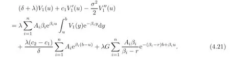
Applying the operatorto both sides,we obtain an(n+2)-th order homogeneous linear differential equation(with undetermined coefficients)for V(u;b).We assume that the roots of the corresponding characteristic equation are distinct.Hence,we get

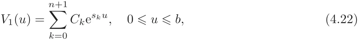
where s0＜ s1＜ ···＜ sn+1and C1,C2,···,Cn+1are undetermined coefficients.

Substituting V1(u)into the original integro-differential equation(4.2),we obtain

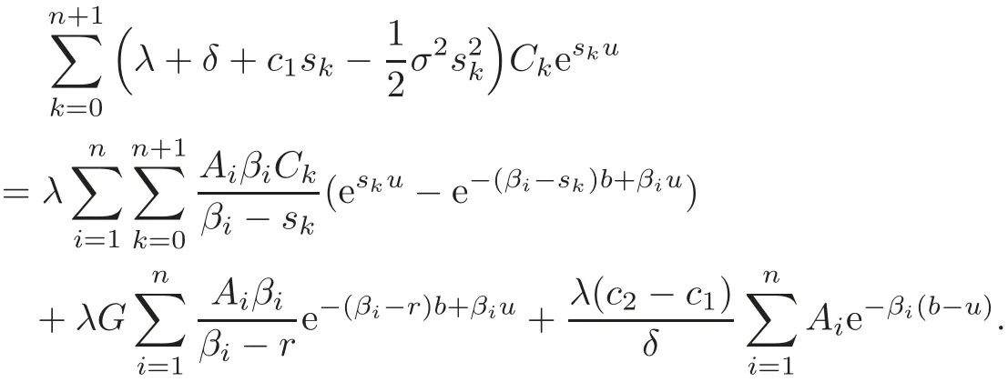
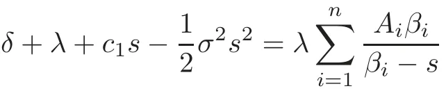
Since the expression above holds for all 0≤ u≤ b,by comparing the coefficients of eskuand eβiu,we obtain

and

Hence,s0,s1,s2,···,sn+1are the roots of

and

Finally,combining(4.24)with the initial condition and the continuity conditions

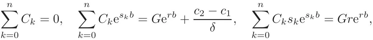
we have a system of n+3 equations to solve C0,C1,···,Cn+1and G.Then the solution for V(u;b)can be expressed as

5 Laplace Transforms

In the last section,we have already calculated V(u;b)purely depending on the integrodifferential equation finished by 0 ≤ u ≤ b and have illustrated the result explicitly for the exponential distribution and mixtures of exponential distributions.Now,we introduce an alternative method for the general cases.

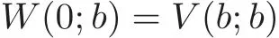
Considering the convolution form in the integral part of(4.2)–(4.3),we apply the Laplace transform to solve V(u;b).In order to discuss the domain of the Laplace transform,we replace the variable u by z=b−u for 0＜u≤b.z denotes the distance between the threshold and the initial surplus,and we define W by

In particular,

and

In terms of the function W(z;b),the integro-differential equation(4.17)becomes

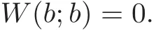
with the initial condition W(0;b)=V(b;b)and the boundary condition W(b;b)=0.

We extend the definition of W by(5.1)to z≥0 and denote the resulting function by w.Then,the equation(5.1)becomes

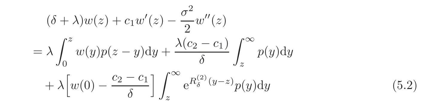
with two constraints w(0)=V(b,b)and w(b)=0.

Letandbe the Laplace transform of w and the density p,respectively.Namely,

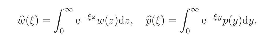
Taking the Laplace transforms in the equation(5.2)for w(z)and p(y),we obtain

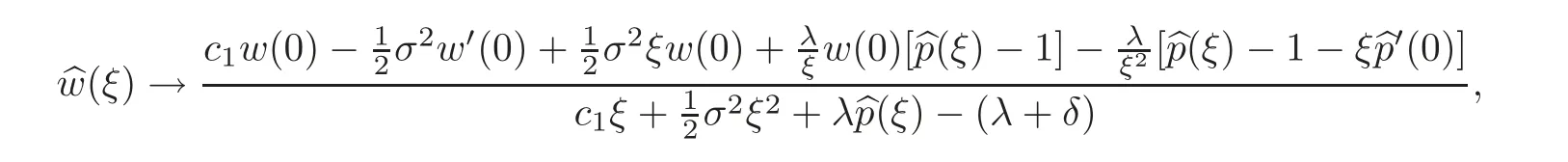
and hence

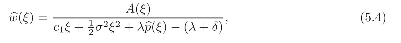
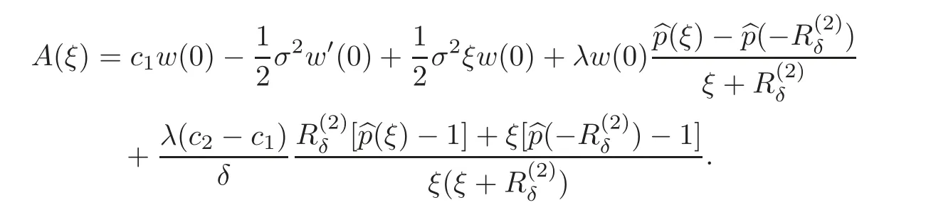
where

We thus have the following procedure for determining V(u;b)and b for a given value of w(0)=V(b;b)and w′(0)=Vu(b;b).Firstly,determine w(z)by the inversion of(5.4).Then the underlying value of b follows from the condition that w(b)=0.Finally,V(u;b)=w(b−u),0≤u≤b.

Remark 5.1 It is easy to see from the graph of

that→ 0 when c2→ ∞.As a result,the limit of the final term in A(ξ)is

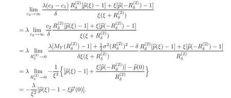
It means that when c2→∞,

which is the Laplace transform of the corresponding w for the barrier strategy(see(4.5)in[5]).Thus,the barrier strategy can be viewed as a limiting case of the threshold strategy.

Remark 5.2 For σ=0,an equivalent result to(7.3)in[4]can be obtained directly.

6 Calculating the Optimal Threshold

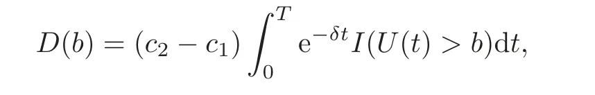
In this section,we study the problem of the determination of the optimal threshold.For a particular value of the initial surplus u,we want to find an optimal threshold level b∗such that the expected total discounted dividends until ruin V(u;b)are maximized.Thus

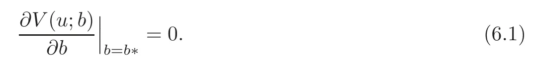
We show how b∗and V(u;b∗)can be calculated below.

If we differentiate the identity Vu(b−;b)=Vu(b+;b),we obtain another identity:

For b=b∗,the second term of both sides vanishes because of(6.1).It follows that

and thus Vuu(u;b∗)is continuous at b∗.This phenomenon is named the high contact condition in finance literature and the smooth pasting condition in the literature on optimal stopping problems.By Remark 4.1 in Section 4,we have

It follows that

By using(4.15)and the above equations,we have

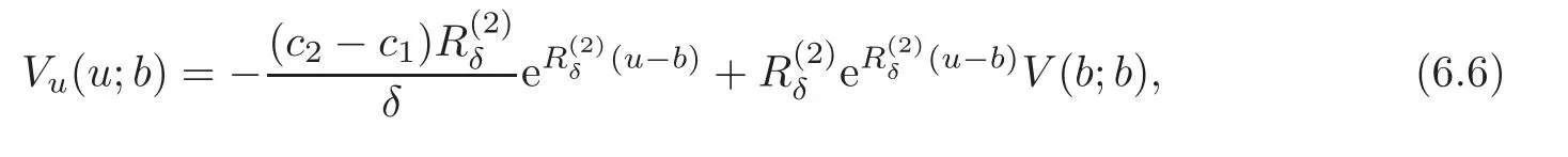
and hence

In fact,the form of V(b∗;b∗)in the exponential case holds for all pro fit distributions.

Remark 6.1 For σ=0,shares exactly the same definition as Theorem 2 in[19].Thus,(6.7)coincides with(25)in[19].

Remark 6.2 By using the definition ofwe can rewrite V(b∗;b∗)as

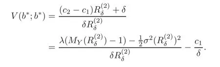
Sincewe obtain

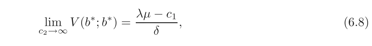
which coincides with(5.9)in[4]and(5.4)in[5].A similar result has been obtained by Gerber[11]for the pure diffusion model.

Now we turn to the problem of determining V(u;b∗)and b∗.Formula(6.7)is crucial for implementing the method of the Laplace transform described in Section 5.Formula(6.7)is equivalent toThus we proceed as follows.In(5.4)we set w(0)=so we obtain the function w(z)by the inversion of its Laplace transform.Then b∗is the zero of w(z),and

Together with(4.15),we can deduce the optimal level of threshold and V(u;b∗)for u ≥ 0.

[1]Alvarez,L.H.R.,Singular stochastic control in the presence of a state-dependent yiels structure,Stoch.Proc.Appl.,86,2000,323–343.

[2]Asmussen,S.and Taksar,M.,Controlled diffusion models for optimal dividend pay-out,Insur.Math.Econ.,20,1997,1–15.

[3]Asmussen,S.,Højgaard,B.and Taksar,M.,Optimal risk control and dividend distribution policies,example of excess-of loss reinsurance for an insurance corporation,Financ.Stoch.,4(3),1999,299–324.

[4]Avanzi,B.,Gerber,H.U.and Shiu,E.S.W.,Optimal dividends in the dual model,Insur.Math.Econ.,41,2007,111–123.

[5]Avanzi,B.and Gerber,H.U.,Optimal dividends in the dual model with diffusion,ASTIN Bulletin,38(2),2008,653–667.

[6]Belhaj,M.,Optimal dividend payments with cash reserves follow a jump-diffusion process,Math.Financ.,20(2),2010,313–325.

[7]Beneˇs,V.E.,Shepp,L.A.and Witsenhausen,H.S.,Some solvable stochastic control problems,Stochastics,4(1),1980,39–83.

[8]B¨uhlmann,H.,Mathematical Methods in Risk Theory,Springer-Verlag,New York,1970.

[9]Chi,Y.C.and Lin,X.S.,On the threshold dividend strategy for a generalized jump-diffusion risk model,Insur.Math.Econ.,48,2011,326–337.

[10]De Finetti,B.,Sur un’impostazione alternativa della teoria collettiva del rischio,Transction of the XVth International Congress of Actuaries,2,1957,433–443.

[11]Gerber,H.U.,Gamnes of economic survival with discrete-and continuous-income processes,Oper.Res.,20,1972,37–45.

[12]Gerber,H.and Shiu,E.S.W.,On the time value of ruin,N.Amer.Actuar.J.,2,1998,48–78.

[13]Gerber,H.and Shiu,E.S.W.,Optimal dividends:Analysis with Brownian motion,N.Amer.Actuar.J.,8,2004,1–20.

[14]Gerber,H.and Shiu,E.S.W.,On optimal dividends:From re fl ection to refraction,J.Comput.Appl.Math.,186,2006,4–22.

[15]Gerber,H.and Shiu,E.S.W.,On optimal dividend strategies in the compound Poisson model,N.Amer.Actuar.J.,10,2006,76–93.

[16]Jeanblanc-Picqu´e,M.and Shiryaev,A.N.,Optimization of the fl ow of dividends,Russ.Math.Surv.,50(2),1995,257–277.

[17]Li,S.,The distribution of the dividend payments in the compound Poisson risk model perturbed by diffusion,Scand.Actuar.J.,2,2006,73–85.

[18]Miyasawa,K.,An economic survival game,J.Oper.Res.Soc.JPN,4(3),1962,95–113.

[19]Ng,A.C.Y.,On a dual model with a dividend threshold,Insur.Math.Econ.,44,2009,315–324.

[20] Øksendal,B.,Stochastic Differential Equations,Springer-Verlag,New York,2006.

[21]Taksar,M.,Optimal risk and dividend distribution control models for an insurance company,Math.Meth.Oper.Res.,51,2001,1–42.

[22]Wan,N.,Dividend payments with a threshold strategy in the compound Poisson risk model perturbed by diffusion,Insur.Math.Econ.,40,2007,509–523.

[23]Wen,Y.Z.,On a class of dual model with divided threshold,Adv.Pure Math.,1,2011,54–58.

[24]Wen,Y.Z.,On a class of dual model with diffusion,Int.J.Contemp.Math.Sci.,6,2011,793–799.