Local Precise Large and Moderate Deviations for Sums of Independent Random Variables∗

Fengyang CHENG Minghua LI

1 Introduction

Throughout this paper,let{X,Xk:k≥1}be a sequence of independent and identically distributed(i.i.d)random variables(r.v.s)with a common distribution F.For some T∈(0,∞],let Δ=Δ(T)=(0,T]if T＜∞and Δ=Δ(T)=(0,∞)if T=∞.In addition,for any real x,we write x+Δ=(x,x+T]if T＜∞and x+Δ=(x,∞)if T=∞.

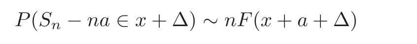
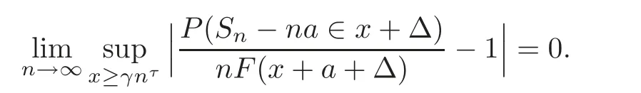
In this paper,we establish some results of the local precise moderate and large deviation probabilities for partial sumswhich state that under some suitable conditions,for some constants T ＞ 0,a and τ＞and for every fixed γ ＞ 0,the relation holds uniformly for all x≥γnτas n→∞,that is,

In the case τ=1,Doney[6],Baltr¯unas[2]and Lin[8]established results of local large deviation probabilities for partial sums,in which X was assumed to be an integer-valued r.v.with a finite mean.Yang et al.[10]gave a result in which X was assumed to be an absolutely continuous r.v.with a finite mean.The results of local large deviation probabilities for which X was assumed to be an integer-valued r.v.with an in finite mean were established by Doney[7].Motivated by the above-mentioned literatures,we establish some results of local precise moderate and large deviation probabilities for partial sums in a unified form in which X may be a type r.v.of an arbitrary.We also discuss the case where X has an in finite mean.

This paper is organized as follows.Section 2 presents notations and definitions of some function classes.Main results are formulated in Section 3.In Section 4,we give some propositions as preparation.The proofs of the main results are presented in Section 5.

2 Definitions and Preliminaries

Throughout this section,f will denote a nonnegative measurable function defined on[0,∞)or(−∞,∞).

First,we introduce some classes of functions.

Definition 2.1 A function f is said to be O-regularly varying(belonging to the class OR)if f is eventually positive(i.e.,f(x)＞ 0 for sufficiently large x)and

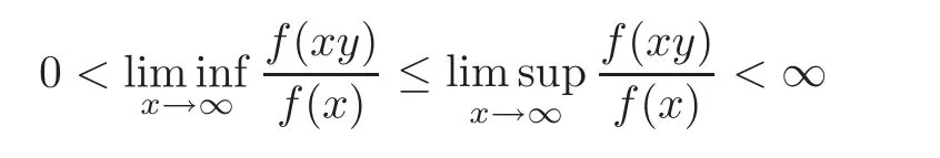
for every fixed y≥1.

If f is an eventually positive function,then its upper and lower Matuszewska’s indices are defined by

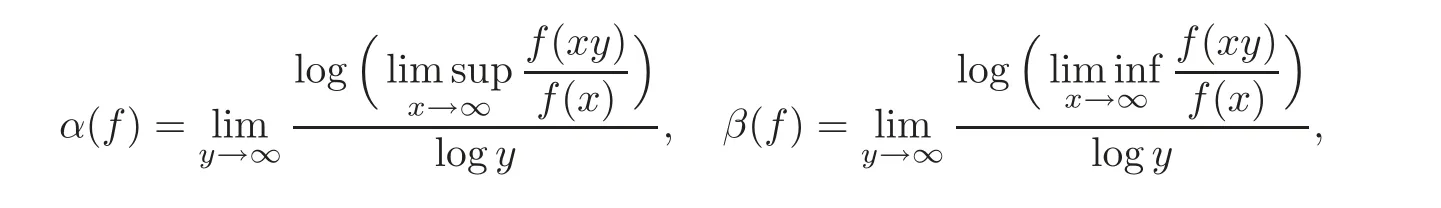
respectively.According to Theorem 2.1.7 in[4],if f is an eventually positive function,then f ∈ OR if and only if its upper and lower Matuszewska’s indices α(f)and β(f)are both finite.

Definition 2.2 A function f is said to be extended regularly varying(belonging to the class ER)if f is eventually positive and

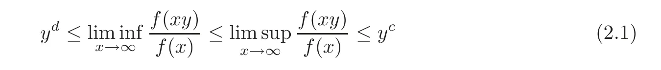
for all y≥1 and some constants c and d,where cd≥0.In particular,if c=d=α in(2.1),then f is said to be regularly varying(belonging to the class R),and it is also said to be regularly varying with index α (belonging to the class Rα).If f belongs to the class R0,then it is said to be slowly varying.

Note that f belongs to the class Rαif and only if f(x)=xαl(x),where l(x)is a slowly varying function.

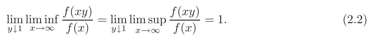
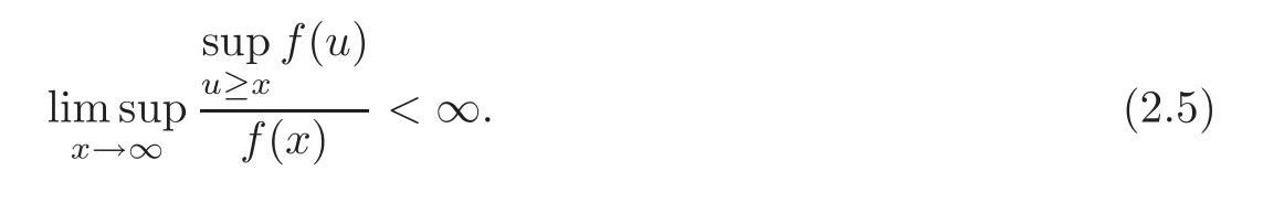
Definition 2.3 A function f is said to be intermediate regularly varying(belonging to the class IR)if f is eventually positive and

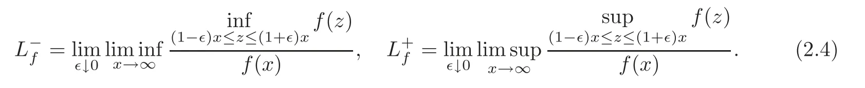
Remark 2.1 By Corollary 2.2 I in[5],if f is eventually positive,then the following are equivalent:

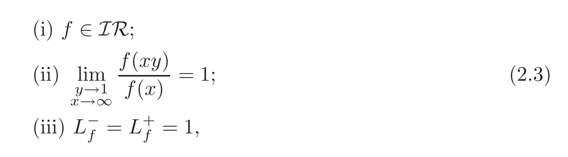
where

If an eventually positive function f satisfies(2.3),then it is also called regularly oscillating,which was introduced by[3].

By Corollary 1.2 in[5],it follows that

and the inclusions are proper.

Definition 2.4 A function f is said to be long tailed(belonging to the class L)if f is eventually positive and

Definition 2.5 A sequence of nonnegative numbers{pn:n=0,±1,±2,···}is said to belong to the class R(or IR,L,ER,OR)if p(x)belongs to the class R(or IR,L,ER,OR),where p(x)is defined by

In the following,we give the definition of almost decreasing,which was introduced by Aljaniand Arandelovi´c[1].

Definition 2.6 A function f is said to be almost decreasing if

Finally,we introduce some notations which will be used in the following sections.Let a(n,x)and b(n,x)be two positive functions(n=1,2,···,x ∈ (−∞,∞)).We denote a(n,x)≾ b(n,x)(or b(n,x)≿a(n,x))which holds uniformly for all x∈Λ as n→∞if

we write a(n,x)∼b(n,x)which holds uniformly for all x∈Λ as n→∞if0.

Obviously,a(n,x)∼b(n,x)holds uniformly for all x∈Λ as n→∞if and only if both a(n,x)≾b(n,x)and b(n,x)≾a(n,x)hold uniformly for all x∈Λ as n→∞.

3 Main Results

In this section,we will present the main results of this paper and give some corollaries.The proofs of the theorem and corollaries are arranged in Section 5.

Theorem 3.1 Let{X,Xk:k≥1}be a sequence of i.i.d.r.v.s.with a common distribution F,and let τ＞be a constant.Suppose that FΔ(x)=F(x+Δ)is almost decreasing,and one of the following conditions holds:

(i)τ≥1,and E(X+)p＜∞for some p＞where X+=max(X,0);or

(ii)τ＜1,and E|X|p＜∞for some p＞

If F(x+Δ)∈OR,then for every fixed γ＞0,the relation

holds uniformly for all x≥γnτas n→∞,where a=EX if τ≤1 and a is any fixed constant if τ＞ 1.Especially,if F(x+Δ)∈ IR,then for every fixed γ ＞ 0,the relation

holds uniformly for all x≥γnτas n→∞,where a is defined as above.

If X is an integer-valued r.v.,by taking T=1,we have the following conclusion.

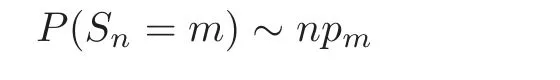
Corollary 3.1 Let{X,Xk:k≥1}be a sequence of i.i.d.integer-valued r.v.s.with the mass pk=P(X=k),k=0,±1,±2,···and let τ＞.Suppose that{pn:n ≥ 1}is almost decreasing and belongs to the class IR.Moreover,Assume that one of the following conditions holds:

(i)τ≥1,and E(X+)p＜∞for some p＞or

(ii)τ＜1 and E|X|p＜∞for some p＞

Then,for every γ＞0,the relation

holds uniformly for all m ≥ γnτas n→ ∞,where a=EX if τ≤1 and a is any fixed constant if τ＞ 1.Especially,if a=0,then for every γ ＞ 0,the relation

holds uniformly for all m≥γnτas n→∞.

Remark 3.1 Note thatimplies that E(X+)p＜∞for some p＞1.Hence,Corollary 3.1 covers Theorem 3.1 in[8].

If X is an absolutely continuous r.v.,then the following conclusion is immediately obtained.

Corollary 3.2 Let{X,Xk:k≥1}be a sequence of i.i.d.r.v.s.with a common almost decreasing density function f.Assume that μ=EX is finite and E(X+)r＜∞for some r＞1.Let γ and T be any fixed positive numbers.If f ∈ OR,then the relation

holds uniformly for all x≥γn as n→∞,where

In what follows,we present an example to show that there is a distribution F with a density f,such that F(x+Δ)∈OR for some T ＞ 0 but f/∈ OR.

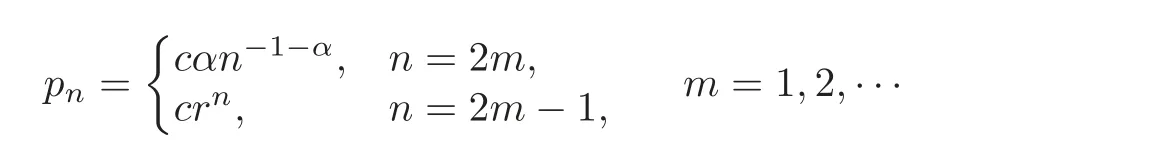
Example 3.1 Let α＞0 and define

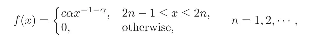
where c is a constant such thatThen,it is clear that f/∈ OR.Let T=2,and then simple calculations yield that

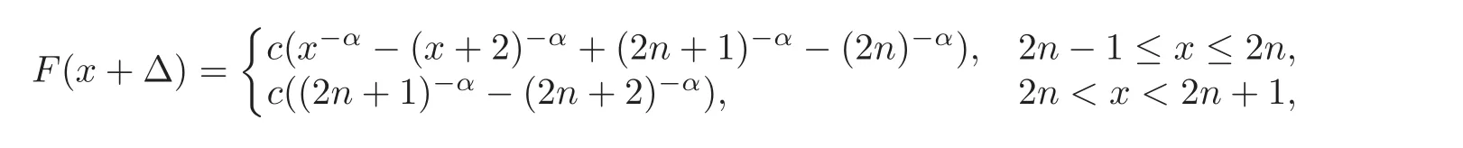
n=1,2,···.It follows that F(x+Δ)∼ cαx−α−1as x → ∞.Thus F(x+Δ)∈ R ⊂ IR ⊂ OR.

Remark 3.2 Example 3.1 and Propositions 4.3–4.5 below show that Theorem 3.1 has a wider range of applications than Theorem 3.1 in[10]even if X has a density function f.

Similarly,there is a lattice distribution F,which has the mass pn=F{n},n=1,2,···,such that F(x+ Δ)∈ OR for some T ＞ 0 but{pn,n=1,2,···}does not belong to OR.

Example 3.2 Let α＞0 and 0＜r＜1.Let F be a distribution with the mass pn,n=1,2,···,where pnis defined by

for some constant c satisfyingThen,it is clear that{pn,n=1,2,···}does not belong to OR,and hence,it does not belong to R.Let T=2,and then simple calculations yield that

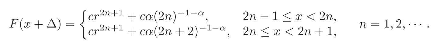
It follows that F(x+Δ)∼cαx−α−1as x→∞,and hence,F(x+Δ)∈R⊂IR⊂OR.

4 Some Propositions

In this section,we give some propositions to investigate the relationships between f∈OR and F(x+ Δ)∈ OR and the relationships amongif a distribution F has a density function f.

First we present some properties of the class OR,which play important roles in the following discussions and can be found in[4].

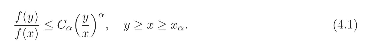
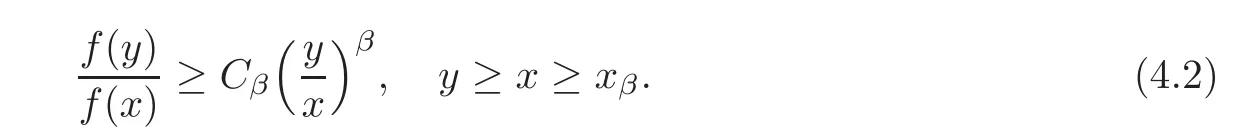
Proposition 4.1 Assume that a function f ∈ OR.Then,for every α ＞ α(f),there exist positive constants Cαand xα,such that

Similarly,for every β ＜ β(f),there exist positive constants Cβand xβ,such that

The following proposition was established by Aljanˇci´c and Arandelovi´c[1].

Proposition 4.2 Assume that a function f∈OR.Then,for any fixed 0＜a＜b＜∞,

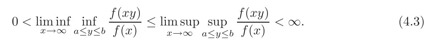
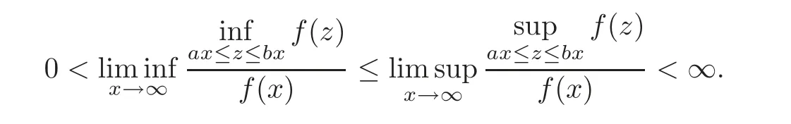
Remark 4.1 It is obvious that(4.3)is equivalent to

The next proposition shows that condition f∈OR is stronger than condition F(x+Δ)∈OR.

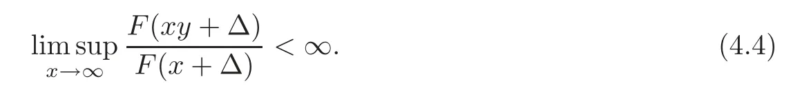
Proposition 4.3 Assume that a distribution F has a density function f and f∈OR.Then,for every fixed T＞0,F(x+Δ)∈OR.

Proof If T=∞,then F(x)=F(x,∞)∈OR follows from Lemma 4.3 of Yang et al.[10].Hence,we only need to discuss the case T＜∞.For any fixed y＞1,by f∈OR,combining with Proposition 4.1,simple calculations yield that

Hence,we only need to estimate the lower bound:Suppose that n−1＜y≤n holds for some integer n＞1.By f∈OR and Proposition 4.2,there exist constants C3and x1＞T,such that

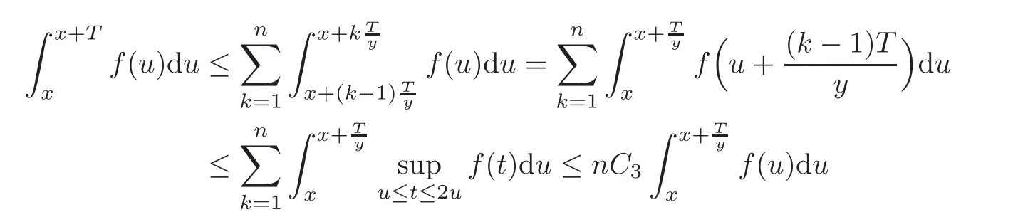
holds for any x＞ x1,where the last but one step is obtained byfor all u≥x≥T and 1≤k≤n.Hence,we have that

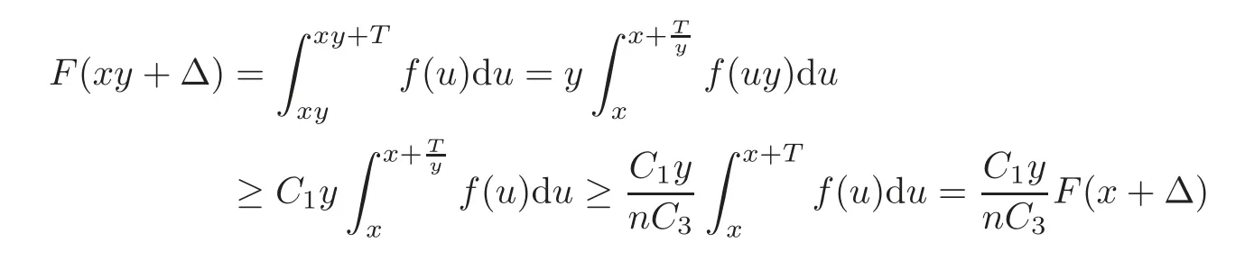
holds for all x＞x1,which yields that

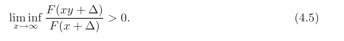
It is obvious that F(x+Δ)∈ OR follows from(4.4)–(4.5).

Proposition 4.4 Assume that a distribution F has a density function f.If f∈OR,then,for every fixed T＞0,

Moreover,if f∈IR,then F(x+Δ)∈IR for every fixed T＞0.

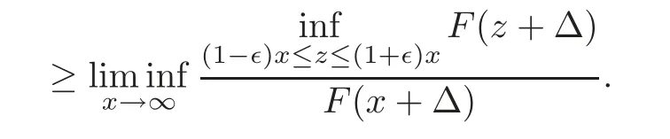
Proof By Proposition 4.2,it follows immediately that＞ 0 and＜ ∞.In what follows,we prove thatBy the definition of,for every fixed δ＞ 0,there exist constants∈0＞0 and x0＞0 such that

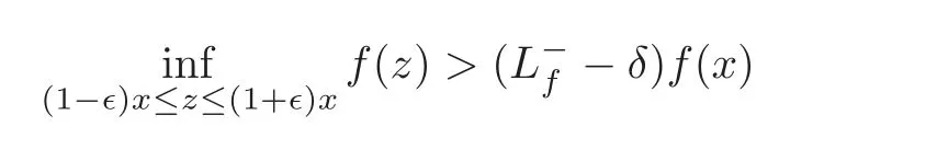
holds for any∈＜∈0and x＞x0.Hence,for any x＞ x0,∈＜ ∈and(1−∈)x≤ z≤(1+∈)x,we have

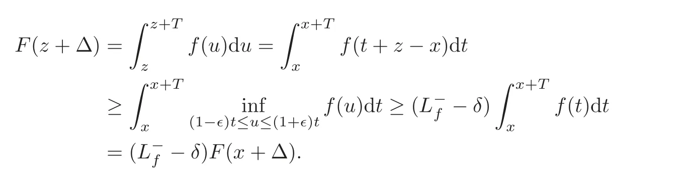
Therefore,

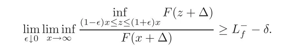
By the arbitrariness of δ,we immediately obtain thatThe proof ofis similar to that ofso it is omitted.

Finally,if f∈IR,then F(x+Δ)∈IR follows immediately from(4.6)and Remark 2.1.

The following proposition shows,the fact that f is almost decreasing implies that F(x+Δ)is almost decreasing.

Proposition 4.5 Assume that a distribution F has a density function f,and f is almost decreasing.Then for every fixed T＞0,F(x+Δ)is almost decreasing.

Proof Since f is almost decreasing,there exist constants C and x0,such thatCf(x)for all x＞x0.We have that

holds for all x＞x0.Hence,F(x+Δ)is almost decreasing.

5 Proofs of Main Results

In this section,we give the proofs of Theorem 3.1 and corollaries.First,we estimate the lower bound of P(Sn−na∈x+Δ)under slightly weaker conditions than those in Theorem 3.1,which will be generalized as Lemma 5.1.

Lemma 5.1 Let{X,Xk:k≥1}be a sequence of i.i.d.r.v.s.with a common distribution F.Suppose thatfor someand FΔ(x)=F(x+Δ)∈ OR.Then for arbitrarily fixed γ＞0,the relation

holds uniformly for all x≥γnτas n→∞,where a=EX if τ≤1 and a is any fixed constant if τ＞1.

Proof Without loss of generality,hereafter we assume that a=0.Since X1,X2,···,Xn,···are i.i.d.r.v.s.,for any fixed∈∈(0,),we have

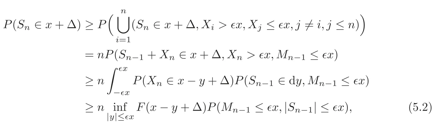
where Mn=max{X1,X2,···,Xn}for all n ≥ 1.Since EX=0 if τ≤ 1,by the strong law of large numbers for i.i.d.r.v.s.,it follows fromthatas n→ ∞.Therefore,Combining with(5.2),it follows that

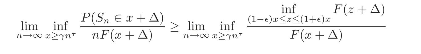
By the arbitrariness of∈,we immediately obtain that(5.1)holds uniformly for all x ≥ γnτas n→∞.

Remark 5.1 The conditions in Lemma 5.1 are slightly weaker than those in Theorem 3.1.In Lemma 5.1,we do not need the condition that F(x+Δ)is almost decreasing.

Now we stand in the position to prove Theorem 3.1.

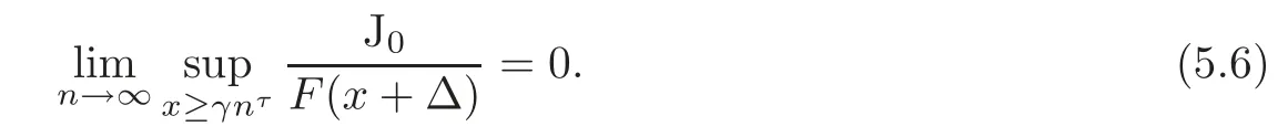
Proof of Theorem 3.1 Without loss of generality,we assume that a=0.By Lemma 5.1,it suffices to prove that

Let v=v(x)= −logF(x+Δ).It is obvious that v(x)is a slowly varying function since F(x+Δ)∈OR andIn fact,for every fixed positive y,

Using the notations similar to Yang et al.[10],we denote

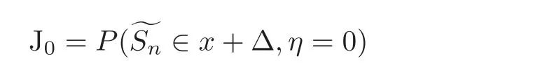
where I(A)is the indicator function of the set A,and letthe(random)number of summands Xi(1≤i≤n)in the sumOur starting point is the decomposition

where

and

We will estimate(5.4)by three steps.

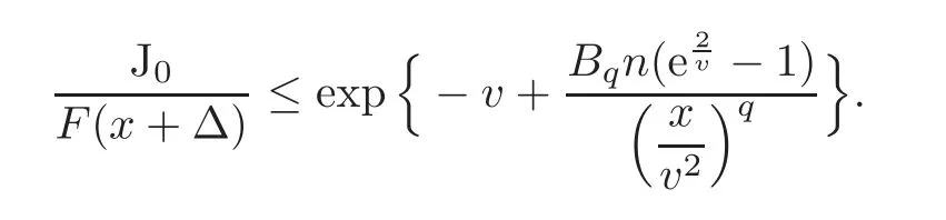
Step 1 Estimation of J0

We use an idea of Tang[9]to deal with J0.For a positive number h=h(x)which will be specified later,by Chebyshev’s inequality,we have

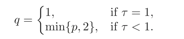
To estimate the upper bound of Eeh?X,we will discuss two cases according to τ＞ 1 and τ≤ 1,respectively.When τ＞1,let q=min{p,1}＞.By virtue of the monotonicity in x∈(0,∞)we obtain that

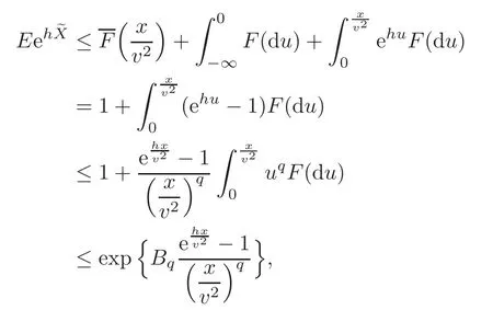
whereHence,we have

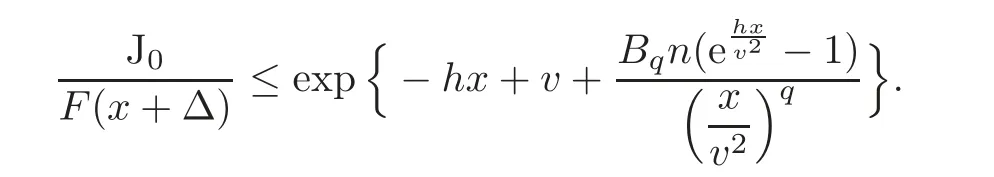
Takingin the above equation,it yields that

Since v(x)is slowly varying and v(x)→∞ as x→∞,combining with qτ＞1,it follows that

When τ≤1,we split eh?Xinto the following several parts:

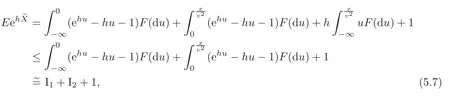
where the last step but one is obtained by EX=0.Let

It is obvious that for 1≤q≤2,the inequality ex−x−1≤|x|qholds for all x＜0.Therefore,and the dominated convergence theorem,it follows that

In what follows,we estimate I2.By virtue of the monotonicity in x ∈ (0,∞)we have

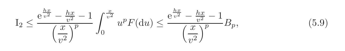
where Bp=E(X+)p＜∞.Substituting(5.8)and(5.9)into(5.7),it follows that

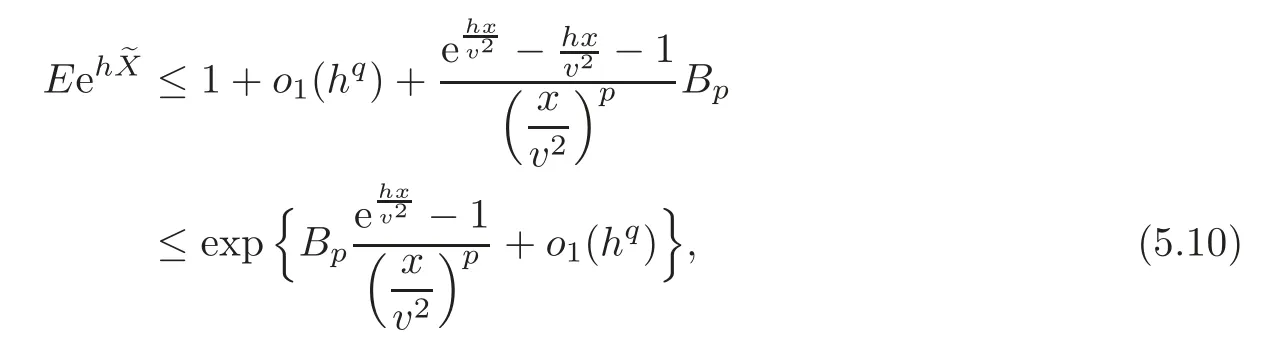
where o1(h)is a real function of h＞0 satisfyingas h→0+.Takingit follows from(5.5)and(5.10)that

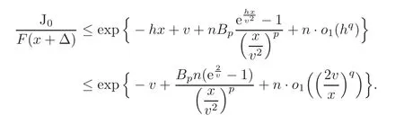
Hence,(5.6)follows since v(x)is slowly varying and v(x)→∞.

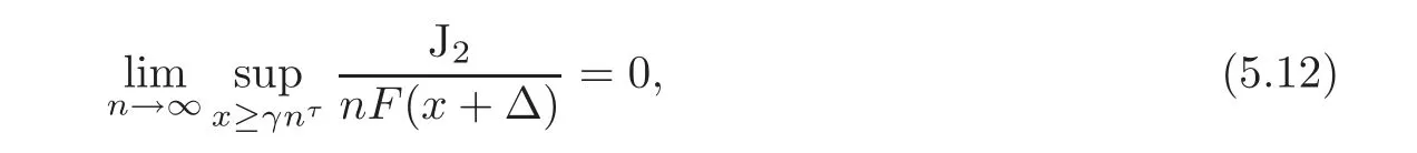
Step 2 Estimation of J2

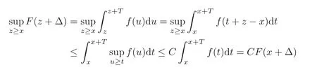
Since X1,X2,···,Xn,···are i.i.d.r.v.s.,for n ≥ 2 and for sufficiently large x,we have that

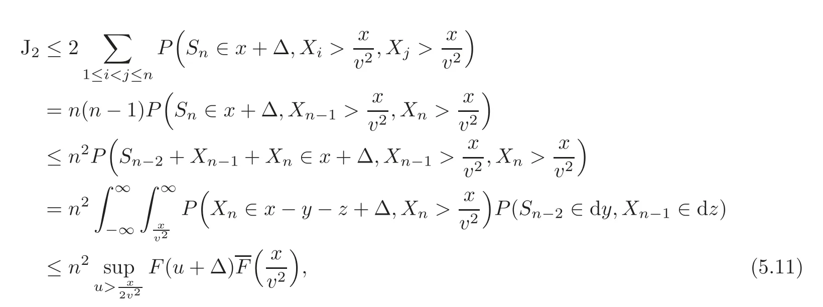
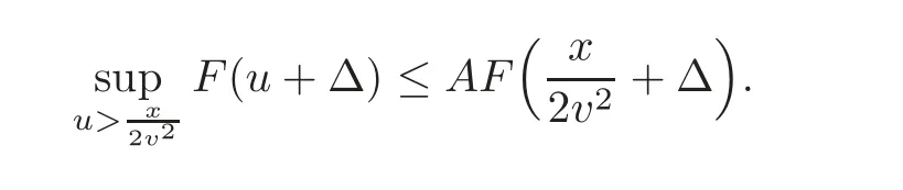
where the last step is obtained by the fact thatholds for alland sufficiently large x if T＜∞,while the inequality is obvious if T=∞.Since F(x+Δ)is almost decreasing,there exist constants A＞0 and x1＞0,for all x＞x1such that

According to Proposition 4.1,for some β ＜ min{β(FΔ),β(F),0},there exist constants Cβand xβ＞ 0,such that

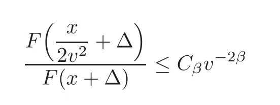
and

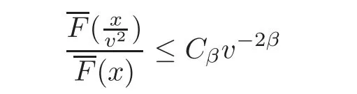
hold for all x satisfyingCombining with(5.11),for sufficiently large x,we have

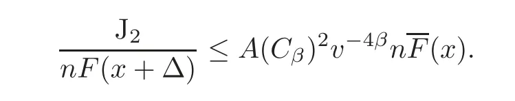
Note that E|X|p＜∞implies thatand that the function v is slowly varying andyield thatas x→∞.Hence,it follows that

sinceholds for x ≥ γnτ.

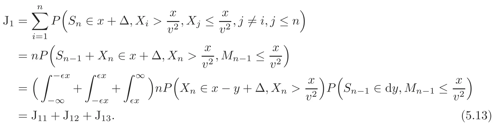
Step 3 Estimation of J1

For every fixed∈∈(0,1),we split J1into three parts as

First,we estimate J11.Since F(x+Δ)is almost decreasing and x−y＞(1+∈)x＞x for all y＜−∈x,there exist constants A and x0,such that

holds for all x＞x0.By the strong law of large numbers of i.i.d.r.v.s.,it follows that

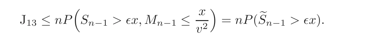
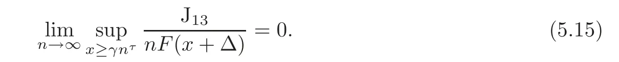
Next,we deal with J13.Clearly,

Hence,it follows from(5.5)–(5.6)that

Finally,we discuss J12.Since(1−∈)x ≤ x−y≤ (1+∈)x for all|y|＜ ∈x,it follows that

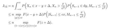
Hence,we have that

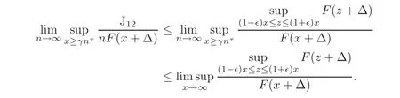
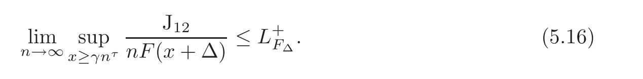
Letting∈↓0,it follows that

From(5.13)–(5.16),we have

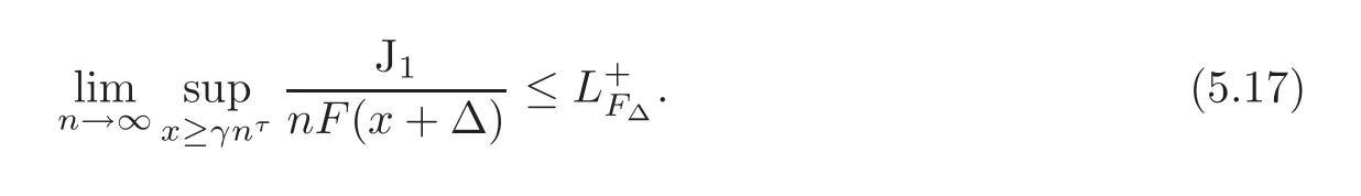
Consequently,(5.3)follows from(5.4),(5.6),(5.12)and(5.17).This completes the proof of the first part of Theorem 3.1.The second part of Theorem 3.1 follows immediately from the first part since F(x+Δ)∈IR implies that

Proof of Corollary 3.1 Taking T=1 and x=m−1 in Theorem 3.1,we have that

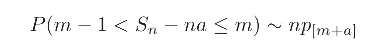
holds uniformly for m≥γnτas n→∞,where[y]denotes the largest integer no more than y.Corollary 3.1 follows since the fact that the sequence{pk:k=0,±1,±2,···}belongs to the class IR implies that the sequence belongs to the class L.

Proof of Corollary 3.2 Corollary 3.2 follows immediately from Theorem 3.1 and Propositions 4.3 and 4.5.

Acknowledgments The authors are grateful to Professor Yuebao Wang and Doctor Dongya Cheng for their useful advice.We would like to thank the anonymous referees for their thoughtful comments on the manuscript.

[1]Aljani,S.and Arandelovi´c,D.,O-regularly varying functions,Publ.Inst.Math.(Beograd),22,1977,5–22.

[2]Baltrnas,A.,A local limit theorem on one-sided large deviations for dominated-variation distributions,Lithuanian Math.J.,36,1996,1–7.

[3]Berman,S.M.,Sojourns and extremes of a diffusion process on a fixed interval,Adv.in Appl.Probab.,14,1982,811–832.

[4]Bingham,N.H.,Goldie,C.M.and Teugels,J.L.,Regular Variation,Cambridge University Press,Cambridge,1987.

[5]Cline,D.B.H.,Intermediate regular and Π variation,Proc.London Math.Soc.,68,1994,594–616.

[6]Doney,R.A.,A large deviation local limit theorem,Math.Proc.Cambridge Philos.Soc.,105,1989,575–577.

[7]Doney,R.A.,One-sided local large deviation and renwal theorems in the case of in finite mean,Probab.Theory Related Fields,107,1997,45–465.

[8]Lin,J.,A one-sided large deviation local limits theorem,Statist.Probab.Lett.,78,2008,2679–2684.

[9]Tang,Q.,Insensivity to negative dependence of the symptotic behavior of precise large deviations,Electron.J.Probab.,11,2006,107–120.

[10]Yang,Y.,Leipus,R.andiaulys,J.,Local precise large deviations for sums of random variables with O-regularly varying densities,Statist.Probab.Lett.,80,2010,1559–1567.