A new approach to quantifying vehicle induced turbulence for complex traf fic scenarios

Yesul Kim ,Li Huang ,Sunling Gong ,2,Charles Q.Jia ,*

1 Department of Chemical Engineering and Applied Chemistry,University of Toronto,200 College Street,Toronto,ON M5S 3E5 Canada

2 Air Quality Research Division,Environment Canada,Toronto,ON M3H 5T4 Canada

1.Introduction

Various computational fluid dynamics(CFD)studies have modeled typical highway conditions using realistic vehicle shapes and compositions and investigated the turbulent kinetic energy(TKE)generated on roadways and its effect on pollutant dispersion[1-3].One difficulty in reproducing realistic roadway conditions using CFD models is simulating two-way traffic.Hu et al.[4]developed a solution procedure,adopting a sliding-mesh approach in which the mesh points are updated as the vehicles move at a specified velocity in opposite directions.They were able to investigate the transient behavior of the air flow in between the two vehicles as w ell as the pressure distributions.How ever,such rigorous approaches are computationally expensive,and their transient nature made it not suitable for highway-scale TKE models.Other studies have suggested different approaches with some simplifying assumptions.One study made an assumption that if the vehicle flow is continuous enough for the TKE to stay constant over time,then a segment of highway can be used as a representative section of the overall highway[1]and vehicles were set to moving w alls with specified velocities.Similar approach has been used by other studies[3].

These studies have built only one set of vehicles for each highway study,claiming that traffic volumes change little between seasons[3]and the traffic composition does not vary much[1].Their works are therefore limited to the specific conditions under which their simulations were set up for,and the results cannot be extended to other roadway conditions.Although the traffic volume may change little between seasons,the hour-to-hour variations were proven to be more significant as shown in field measurements[5,6].Also,these studies were not able to capture the different vehicle-vehicle interactions and its effect on TKE generation,or its decay characteristics,although these factors could be important in determining the fate and transport of air pollutants.One study show ed how the pollutant dispersion and turbulent mixing are impacted by building arrays and packing density in street canyon environments[7].Impacts of similar significance may be expected from different arrays and densities of vehicles on roadways.Sinceit is important that the results are taken and applied beyond the simulation domain,the current study aims to provide insights into different factors that may affect TKE on roadways and to develop parameterizations that can be applied in future studies.

2.Methodology

The commercial Computational Fluid Dynamics(CFD)package,FLUENT,was used in this study.FLUENT is a multi-purpose fluid dynamics software package,which has been widely used in complex air flow and pollutant dispersion applications in various environments.All of the governing equations are discretized using the finite volume method and are solved by using the SIMPLE(Semi-Implicit Method for Pressure-Linked Equation)algorithm in FLUENT,which uses a relationship between velocity and pressure corrections to enforce mass conservation and to obtain the pressure field[8].

2.1.Quantification of vehicle induced turbulence(VIT)

The turbulent kinetic energy(TKE)of the air flow was used to quantify the vehicle induced turbulence(VIT).TKE is defined as the sum of the kinetic energy of the velocity fluctuations.The velocity u may be expressed as:

where ū is the time-averaged mean velocity,and u′is the fluctuating part of the velocity that differs from the average value.

Then the TKE per unit mass of the flow can be expressed as:

where u,v,and w are the fluctuating velocity components in x,y,and z directions.

Since the instantaneous values of TKE can vary dramatically,a mean TKE value is often calculated to represent the overall flow.

Although it is not possible to exactly predict the random and irregular details of turbulent flow,various models have been developed to provide “closure”to the equations governing the average flow.The standard k-ε turbulence model is one of the most widely used and validated CFD turbulence model[1-3,9-11].It offers a good compromise between result accuracy and computational cost in the absence of swirling flow[8].The assumptions used in this model are that the flow is fully turbulent and the effects of molecular viscosity are negligible.

2.2.Simulation setup

2.2.1.Simulation domain and mesh setup

In order to model a realistic roadway condition,three different types of vehicles were used in this study(Fig.1):a passenger vehicle,a sport utility vehicle(SUV),and a truck,which were modeled in real-shape rather than block-shape,since the block-shaped vehicles are estimated to produce 25%more turbulence than real-shaped vehicles[12].Vehicle dimensions are given in Table 1.These vehicles were set to travel along the x-axis,while the y-axis is the width of the domain going into the screen,and the z-axis is the height of the domain.

Fig.1.Shapes of three different types of vehicles:a passenger vehicle,an SUV and a truck.

Table 1 Vehicle dimensions

The domain size in this study was fixed at 100 m×20 m×20 m in x,y,z directions,respectively.This was to compare the volume-averaged TKE w hen there are multiple vehicle interactions,changes in traffic densities and changes in traffic compositions.The computational domain was meshed using ICEM-CFD—a software widely used for generating meshes.To maintain a proper balance between results accuracy and computational expense,variable mesh size was used.Since the gradients in the model variables are more steep right around the vehicles and in the vehicle wake region, finer mesh density was used around the vehicles,and the mesh size was set to grow at a certain ratio as it moves away from the vehicles.Up to 6 million cells were created in each mesh setup.Fig.2 show s a typical mesh setup w here the fine mesh density is shown right around the vehicle;note that there are volume meshes that fill the w hole domain but only the surface meshes are show n here and also that some surfaces are left invisible for the ease of view.More specifically,the smallest grid size was 1 cm around the vehicle tailpipes.The expansion ratios were 1.2 and 1.3 for inner and outer density regions as show n in Fig.2.The mesh size near the ground shares the same parameters as described above.In addition,sensitivity tests were conducted to ensure that two density regions were adequate to obtain relatively constant volume-averaged TKE around a single passenger vehicle.The orders of numerical schemes used in this study are standard for pressure and second order upwind for momentum,TKE and turbulence dissipation rate.The convergence criteria are 10-3for continuity,velocity components,TKE,turbulence dissipation rate and 10-6for energy.

Fig.2.Mesh density setup around a single passenger vehicle.

2.2.2.Boundary conditions

Movement of the vehicles in a steady-state flow was simulated by modeling the vehicles as moving w alls with specified translational velocities in x-direction.For the vehicle surface,an equivalent roughness height of 0.0015 m was used[3];while the ground was set as a stationary wall with a surface roughness of 0.01 m.The road is not raised and there is no barrier or obstacle to air flow,other than the surface roughness.Non-slip boundary conditions and a specified surface temperature(300 K)were applied to the vehicle and the ground surfaces.

As shown in Fig.3,the symmetric boundary conditions were applied to the two side faces and the top face;which means that there is zero gradient in the variables normal to these surfaces,and that there is no flux of all quantities across these surfaces.The front side was modeled as a velocity inlet with zero velocity;while the back side was modeled as an out flow with zero normal first derivatives of all quantities,which means that there is bulk flow only and no diffusive flux for all flow variables in the direction normal to the plane.When external w ind was introduced,the side from which the w ind blow s from was also treated as a velocity inlet,with specified wind velocity components.For the “velocity inlet”boundary in Fig.3,the actual velocity was set to zero,due to no external w ind assumption described in the manuscript.Then,the solution was initialized from vehicles,with absolute reference frame,by specifying moving w all speed of 28 m·s-1(or 100 km·h-1of vehicle traveling speed).

Fig.3.Boundary conditions for the case without ambient wind.

It should be pointed out that this work uses the standard w all function.It is known that the SKE model with the standard w all function will result in an over production of TKE in the near-wall region.The analysis done in this study is based on volume-averaged TKE,which takes into account a great number of grid cells.This over production of TKE is only found in the second above the ground.Therefore,its impacts on our over analysis are minimized while using volume-averaged TKE in the 3 m×20 m×100 m domain.

2.3.Simulation scenarios

For illustrative purpose,the simulation domain and geometry setup for the 6 passenger vehicles case is given in Fig.4.For multiple vehicle cases,all the vehicles were treated as moving w all boundary.It was assumed that all the vehicles were traveling at the same speed of 100 km·h-1.

Fig.4.Computational domain setup for traffic density of 6 passenger vehicles.

2.3.1.Vehicles traveling in series

A single passenger vehicle traveling at 28 m·s-1(or 100 km·h-1)was used as a base case.Then,a second passenger vehicle was added directly behind the first vehicle,and the distance between the two vehicles traveling in series was varied from 1,1.5,2,3 and 5 multiples of body length,w here the body length of the passenger vehicle is 4.5 m.The distance between the inlet face and the first vehicle is 10 m.

2.3.2.Vehicles traveling side-by-side

Again,a single passenger vehicle with velocity 28 m·s-1was used as a base case,and a second vehicle was added next to the first vehicle,traveling in the same direction.The distance between the two side by-side traveling vehicles were varied from 1,1.5 and 2 multiples of body width for 2 passenger vehicle cases;1 body width for 1 passenger vehicle and 1 SUV case;and 1 body width for 1 passenger vehicle and 1 truck case;w here the body width of the passenger vehicle is 1.8 m.For the cases of different vehicle body lengths,the centerline of the vehicles was matched to represent a side-by-side position.

2.3.3.Vehicles traveling in opposite directions

The effect of vehicles traveling in opposite directions was studied in this section.The vehicles were treated as moving walls with velocities in the opposite directions.Two passenger vehicles were set to travel in the opposite directions,while the distance between them was varied from 1 to 2 multiples of body width,1.8 m.

2.3.4.Traffic density

The traffic density was varied from 1,2,4,6,to 8 passenger vehicles evenly spaced out in the computational domain.Similar steps were taken with increasing number of trucks in the absence of passenger vehicles.The number of trucks in the domain was increased from 1,2,to 3.Only one type of vehicle was used in each part,as the effect of traffic composition is studied in a separate section.As will be show n in later sections,the effect of side-by-side interaction of vehicles traveling in opposite directions is not significant on the overall TKE in the computational domain,therefore the traffic density studies were carried out in one-way traffic only.The axis orientation,scale,and the relative spacing of the vehicles can be seen in Fig.4.

2.3.5.Traffic composition

Different traffic compositions were simulated with increasing number of trucks,while keeping the total number of vehicles constant at 8 vehicles.The cases simulated were 1 truck and 7 passenger vehicles;2 trucks and 6 passenger vehicles;and 3 trucks and 5 passenger vehicles.For the same reason described in the traffic density cases,only one-way traffic was simulated.

3.Results and Discussion

3.1.Effect of distance between vehicles

3.1.1.Vehicles traveling in series

Fig.5 show s the TKE contour on the xz-plane when two vehicles are traveling in series.TKE values have been plotted against the distance be hind the first vehicle along the centerline of the vehicle at vehicle top height.The results are presented in Fig.6.Zero on the x-axis corresponds to the end of the first vehicle,thus the peak that appears before zero is above the body of the first vehicle.

It can be seen that as the second vehicle drives into the TKE wake region created by the vehicle in front,the TKE behind the second vehicle peaks up.As the distance between them increases,the TKE generated by the first vehicle is allow ed to decay further down before the second vehicle approaches it,but as the second vehicle drives in,the TKE value is superimposed on the existing TKE value at the point.At about 5 body lengths apart,the effect of the first vehicle is not significant anymore,and the peak produced by the second vehicle is as high as the peak produced by the first vehicle.

The volume-averaged TKE values are calculated for each of the case,under a mixing height of 3 m and the result is presented in Table 2.The volume-averaged TKE value for a single passenger vehicle case is listed as a base case for comparison.

Fig.5.TKE contour on xz-plane for two passenger vehicles in series.

Fig.6.TKE vs.distance behind the 1st vehicle for different distances between vehicles in series.

Table 2 Volume-averaged TKE for passenger vehicles traveling in series with different distances between them

Comparing the single passenger vehicle case to two passenger vehicles cases,it can be seen that the volume-averaged TKE values are not simple multiples of the vehicle numbers,since the second vehicle travels into the first vehicle's wake region of elevated TKE.The relationship between the number of vehicles and the average TKE is to be discussed in detail later.

Considering the volume-averaged TKE values for the two-vehicle cases with different distance between them,the volume-averaged TKE values remain constant regardless of the distance between the two vehicles.This means that the TKE values are linearly superimposed w hen the second vehicle travels into the TKE wake region created by the first vehicle,and there are no other interactions that would further change the value of the average TKE.Note that the volume-averaged TKE value for 5BL-apart case is lower than the other cases.This is because the second vehicle is located very far behind the first vehicle;thus a significant portion of the TKE wake behind the second vehicle is located outside the computational domain,resulting in lower average TKE value.

3.1.2.Vehicles traveling side-by-side

TKE generation was simulated for two passenger vehicles traveling next to each other at various distances apart.Fig.7 show s the TKE value plotted along a line that runs behind the vehicle through the center of one of the vehicles.It can be concluded that there is little impact on the TKE behind one of the vehicles,even if there is another vehicle traveling next to it.The same can also be said from the TKE contour show n in Fig.8.TKE wake regions do not extend far in the lateral direction;as a result,one vehicle's wake region has very little impact on another vehicle's.

Fig.7.TKE vs.distance behind a vehicle:for different distances between side-by-side vehicles.

Then,the effect of having different types of vehicle in the adjacent lane was simulated.The distance between the two vehicles was fixed at 1 body width(1.8 m);while the type of vehicle in the adjacent lane was changed from a passenger vehicle to an SUV and then to a truck.Fig.9 show s the TKE value plotted along a line that runs through the center of the passenger vehicle as distance increases away from the vehicle,and the height at the top of the vehicle.It is clear that even for the case of a truck in the adjacent lane,there is not a significant change in the TKE wake region behind a passenger vehicle.As can be seen on the TKE contour in Fig.10,the TKE wake region does not extend very far in the lateral direction,so the side-by-side interaction is not significant even when there is a truck in the adjacent lane.

3.1.3.Vehicles traveling in opposite directions

Fig.11 compares the two cases when the distance between the two passenger vehicles is 1.5 times the body width;one case is when the two vehicles are traveling in the same direction and the other case is w hen they are traveling in the opposite directions.It is clear that there is not a significant difference between the two cases being compared.It has been determined previously that the horizontal interaction between the vehicles is small when they are moving in the same direction;the same can be said for the vehicles moving in the opposite directions.

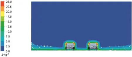
Fig.8.TKE contour on yz-plane for two passenger vehicles traveling in adjacent lanes.

Fig.9.TKE vs.distance behind a passenger vehicle:for different types of vehicle in the adjacent lane at 1 body-width apart.

Fig.12 compares TKE values plotted against the distance behind one of the two vehicles,w hen the other vehicle is traveling in the opposite direction in the next lane at various distances away.The initial TKE values are similar for all three cases.It is only after about 15 m that there is a slight difference:when the vehicles are very close together only at 1 body-width apart,the resulting TKE is slightly higher in the far field compared to the cases w hen the vehicles are further apart at 1.5 or 2 body-widths apart.To see how significant this difference is,the volume-averaged TKE was calculated for the cases with various separation distances,for both the same and the opposite traveling directions.Again,a mixing height of 3 m was used.

From Table 3,it can be concluded that there is not a big difference in the volume-averaged TKE values when these vehicles are moving in the same direction or in the opposite directions,as the difference in volume-averaged TKE bet ween the cases does not exceed 5%.This result con firms the earlier conclusion that there is a very little horizontal interaction,regardless of the vehicles' travel direction,vehicle types,and the distance between them.

Fig.11.TKE vs.distance behind one of the two passenger vehicles traveling at 28 m·s-1 in the same or in the opposite directions.

3.2.Effect of number of vehicles in the domain

In this section,the effect of the number of vehicles in the domain,or traffic density,on the overall volume-average TKE was determined.The number of passenger vehicles was increased from 1 to 2,4,6,and 8 in the absence of trucks;and the number of trucks was increased from 1 to 2,and then to 3 in the absence of passenger vehicles.Since it has been found in the previous sections that the travel directions do not have a significant impact on the average TKE in the domain,the vehicles were all set to travel in the same direction.The volume-averaged TKE under a mixing height of 3 m has been plotted as a function of the number of passenger vehicles and number of trucks in the domain.The data was fitted using linear equations as show n in Fig.13.

Fig.10.TKE contour on yz-plane for one passenger vehicle and one truck traveling in adjacent lanes.

Fig.12.TKE vs.distance behind one of the two passenger vehicles traveling at 28 m·s-1 in the opposite directions,at different horizontal distance apart.

Table 3 Volume-averaged TKE for two passenger vehicles traveling in adjacent lanes

Fig.13.Volume-averaged TKE vs.number of vehicles in the domain under mixing height of 3 m.

The equations for the passenger vehicle and truck derived from this study are:

These two equations relate the volume-averaged TKE under a mixing height of 3 m,on a 100 m(x-direction)by 20 m(y-direction)segment of the road,with increasing number of each type of vehicle.All of the vehicles are set to travel at 28 m·s-1in the positive xdirection.The absolute values of slop and intercept in the above equations vary with the dimensions of averaging volume,road characteristics,and vehicles' traveling speed.

The slopes indicate the incremental change in the volume averaged TKE with increasing number of each type of vehicle,and the y-intercept values represent the road-induced turbulence(RIT).Theoretically,the RIT values for the passenger vehicles and the trucks should be very similar,but the y-intercept values obtained for passenger vehicles and trucks from this study are different.This could be due to a possible limitation in the size of the computational domain,especially with the trucks because of their lengths.When there are multiple trucks in the domain,a fraction of the TKE wake region behind the last truck happens to be located outside the domain,resulting in a lower TKE value.This could have affected the values of the slope and y-intercept of the equation.

3.3.Effect of traffic composition in the domain

This section analyzes the effect of traffic mix,or traffic composition,on the volume-averaged TKE in the domain.The number of trucks in the domain was increased from 0 to 3 while the number of passenger vehicle was decreased from 8 to 5,thus keeping the total number of vehicles constant at 8.

Fig.14 show s the TKE contour of the case where there are2 trucks in the domain.There is a zone of high TKE created behind the first truck,same as the case with a single truck.TKE decays down with the distance behind the first truck as expected,then increases to a certain extent,affected by the two passenger vehicles,and there is a zone of relatively low TKE before the second truck drives in.Behind the second truck,there is a zone of high TKE created.

Not much can be said from the contour alone;therefore the volume-averaged TKE values are compared.Since there are trucks in addition to passenger vehicles,a mixing height of 4 m was also considered as w ell as the usual 3 m.The two results are plotted on the same axis as show n in Fig.15.

The two graphs for different mixing heights show similar results,with only a small difference in values.Mixing height of 4 m was able to capture some of the high-rising TKE wake zones,resulting in a higher average TKE values than that under a mixing height of 3 m.These two graphs both show that there is a large increase in volume-averaged TKE when the first truck is added,how ever,additional increments in the number of trucks do not cause as a large increase in TKE as the first truck does.

To predict the change in the volume-averaged TKE with a change in traffic composition,Eqs.(4)and(5)relating the number of vehicles to the volume-averaged TKE in the domain are used.Assuming independent contribution from the passenger vehicles and the trucks,the equations are simply superimposed.The y-intercept value for passenger vehicles and the y-intercept value for trucks are averaged,to represent the “average”RIT,and the slope for each type of vehicle was used.

The resulting equation is:

Using this equation,the volume-averaged TKE values are calculated for different traffic compositions,and the calculated values are compared to the simulated values in Fig.16.

Fig.14.TKE contour on xz-plane for two trucks and multiple passenger vehicles.

Fig.15.Volume-averaged TKE for different traffic compositions in the domain under mixing height of 3 m and 4 m.

Fig.16.Simulated vs.calculated volume-averaged TKE for different traffic compositions in the domain under mixing height of 3 m.

Overall,the simulated values and the calculated values are reasonably close in values.For the case with 7 passenger vehicles and 1 truck,the calculated value is 9%lower than the simulated value,which could be due to an error introduced from using the average RIT value.For the case with 5 passenger vehicles and 3 trucks,the calculated TKE is about 16%higher than the simulated TKE.This difference could be due to,in addition to the error from the RIT value,the limit in the size of the computational domain.As the traffic density increases in the domain,some of the vehicles are located too far back in the domain,and the TKE regions created behind them are not fully captured in the calculation as they happen to be located outside the domain.This error could be reduced if a larger domain size is used.Despite the difference,it seems that the independent contribution from each type of vehicles may be added together to yield a reasonable estimation of the overall volume averaged TKE in the domain w hen there are different traffic compositions on road.

4.Conclusions and Implications

The current study provides insights into w hat are the key factors in estimating TKE in the domain of interest and has resulted in following findings:

(1)It was show n for the first time that the overall VIT from multiple vehicles traveling in series can be estimated by superimposing the VIT of each vehicle,without considering the distance between them while the distance is greater than one vehicle length.This finding is particularly significant since it enables a new approach to VIT simulations w here the overall VIT is calculated as a function of number of vehicles.

(2)Since the TKE wake does not extend very far perpendicular to the road the interactions between vehicles traveling next to each other in adjacent lanes are not significant,regardless of the directions of the traffic flow.Consequently,simulations of different traffic scenarios can be substantially simplified by treating two way traffic as one-way traffic,which would result in less than 5%difference in the overall volume-averaged TKE.

(3)For any single type of vehicles,the volume-averaged TKE in the mixing zone can be expressed as a linear function of the number of vehicles in the domain.The following equation can be used to relate the number of passenger vehicles or trucks to the volume averaged TKE under a mixing height of 3 m.

(4)With different types of vehicles in the domain how ever,the relationship between the volume-averaged TKE is no longer linear with an increase in the total number of vehicles.The contribution from each vehicle type needs to be treated separately,and the linear expression for each vehicle is summed up to yield the total volume-averaged TKE.For the case of trucks and passenger vehicles,volume-averaged TKE was estimated by the following equation:

Acknowledgments

We acknowledge the financial support from Environment Canada and the Government of Ontario(72021622)for a scholarship to YK.

[1]Ali M.Sahlodin,Rahmat Sotudeh-Gharebagh,Yifang Zhu,Modeling of dispersion near roadways based on the vehicle-induced turbulence concept,Atmos.Environ.41(1)(2007)92-102.

[2]Efisio Solazzo,Xiaoming Cai,Sotiris Vardoulakis,Modelling wind flow and vehicleinduced turbulence in urban streets,Atmos.Environ.42(20)(2008)4918-4931.

[3]Y.Jason Wang,K.Max Zhang,Modeling near-road air quality using a computational fluid dynamics model,CFD-VIT-RIT,Environ.Sci.Technol.43(20)(2009)7778-7783.

[4]Xingjun Hu,Fu.Limin,Baoqin He,Sheng Li,Yingchao Zhang,Yunzhu Wu,Numerical simulation of three dimensional transient aerodynamic characteristics of two crossing vehicles,Int.J.Comput.Methods Eng.Sci.Mech.8(2007)223-231.

[5]Jie Lin,Dan Yu,Traffic-related air quality assessment for open road tolling highway facility,J.Environ.Manag.88(4)(2008)962-969.

[6]Mark Gordon,Ralf M.Staebler,John Liggio,Paul Makar,Shao-Meng Li,Jeremy Wentzell,Gang Lu,Patrick Lee,Jeffrey R.Brook,Measurements of enhanced turbulent mixing near highways,J.Appl.Meteorol.Climatol.51(9)(2012)1618-1632.

[7]Di Sabatino Silvana,Riccardo Buccolieri,Beatrice Pulvirenti,Rex Britter,Simulations of pollutant dispersion within ideal is ed urban-type geometries with CFD and integral models,Atmos.Environ.41(2007)8316-8329.

[8]ANSYS.Inc.,ANSYS FLUENT User's Guide,2010.

[9]Jaroslav Katolický,Miroslav Jicha,Eulerian-Lagrangian model for traffic dynamics and its impact on operational ventilation of road tunnels,J.Wind Eng.Ind.Aerodyn.93(1)(2005)61-77.

[10]Dong-Hee Kim,Mridul Gautam,Dinesh Gera,On the prediction of concentration variations in a dispersing heavy-duty truck exhaust plume using k-epsilon turbulent closure,Atmos.Environ.35(31)(2001)5267-5275.

[11]J.S.Wang,T.L.Chan,C.S.Cheung,C.W.Leung,W.T.Hung,Three-dimensional pollutant concentration dispersion of a vehicular exhaust plume in the real atmosphere,Atmos.Environ.40(3)(2006)484-497.

[12]Roger S.Thompson,Robert E.Eskridge,Turbulent-diffusion behind vehicles—experimentally determined influence of vortex pair in vehicle wake,Atmos.Environ.21(10)(1987)2091-2097.