The Classification of the High Resolution Remote Sensing Images with BKNNSVM



The Classification of the High Resolution Remote Sensing Images with BKNNSVM

ShuZhenyu1,ZhouCheng1,WangDianhong2

(1 College of Electronics and Information, South-Central University for Nationalities, Wuhan 430074, China; 2 Institute of Geoscience & Geomatics, China University of Geosciences, Wuhan 430074, China)

AbstractIn order to solve the deficiency about the algorithm of the local support vector machine (KNNSVM) which is very time-consuming on classifying the high resolution remote sensing images with mass data and improve the performance of the KNNSVM, the BKNNSVM algorithm based on uncertainty is proposed. The algorithm applies the binomial distribution of conjugate prior Beta distribution to estimate probability belong to the class or negative of each unlabeled sample through its nearest neighbor distribution. Then, with threshold, some unlabeled samples are classified by the KNN when their uncertainty value is less than threshold and others are classified by the local SVM when their uncertainty value is more than threshold. The experiments on the actual high resolution remote sensing images have shown that BNNSVM can decrease the time consuming effectively and keep the precision of the original KNNSVM with suitable threshold of uncertainty.

Keywordshigh resolution remote sensing images; KNNSVM; BKNNSVM

With the rapid development of communication technology, the remote sensing image shows the trend with higher and higher resolution. The remote images with higher resolution contain rich information which can promote the more applications of the remote images in the practice fields. Therefore, the high resolution remote sensing images have become an important source to recognize the ground objects. On the other hand, the higher resolution of the remote sense images resolution and the demand of the accuracy with the remote sense images in the application fields have become a great challenge for experts to deal with them. With the improvement of its have increased, the data which need to be processed increased exponentially. As a result, the traditional image processing[1]mode relied on artificial visual interpretation has been unable to satisfy the practical needs, the remote sense images′ automation classification with computer such as data mining and machine learning[2-4]have become the main method.

Support vector machine (SVM)[5]which is established by the support vectors with advantages of good sparse, high accuracy and quick running speed is a classification model. For the sake of its features, it is very suitable to process the classification problems with small training data, nonlinear and high dimension. Consequently, it is widely applied in the remote sense images classification fields[6-8].

However, the traditional Support Vector Machine does not satisfy the global consistency which leads to the lower accuracy when it is applied to classify some samples. In order to further improve classification performance, especially to meet the requirements of global consistency, the Local Support Vector Machine algorithm had been proposed and widely applied in the practice fields. The Local Support Vector Machine algorithm was first proposed by Brailovsky et al.[9]on

1999. They realized the locality of the traditional SVM by adding two multipliers to the kernel functions. To compensate the deficiency of the Local Multipliers Support Vector Machine, Zhang et al[10]had proposed the algorithm SVM-KNN. The classical Local Support Vector Machine algorithm KNNSVM was proposed by Blanzicrii and Melgani[11]for further improving performance. To further optimize the algorithm of KNNSVM, LSVM[12], PSVM[13]and Falk-SVM[14]were all proposed.

Although the Local Support Vector Machine algorithm has made great progress, because of the convergence of KNN algorithm and SVM algorithm, it has features of high classification accuracy and much time consumption. In order to make up the deficiency of the traditional Local Support Vector Machine, we propose the algorithm BKNNSVM which decrease the time consuming of KNNSVM based on Beta distribution. The experimental results show that the algorithm BKNNSVM can decrease time consumption obviously and has the similar accuracy comparing to the algorithm KNNSVM when the threshold is reasonable.

1Analysis of the algorithm KNNSVM

KNNSVM[11]algorithm is developed from the algorithm SVM-KNN. Compared to the SVM-KNN, KNNSVM directly finds K neighbors in the linear kernel space which avoided the nonlinear phenomena of the distance measure on some classification problems. The connections between the neighbors and the unlabeled samples are more closely related, and at the same time, KNNSVM is more direct viewing for not needing to transform the distance matrix.

1.1Description of the algorithm KNNSVM

The algorithm KNNSVM is described as below.

(1) As to the unlabeled samplex′，we calculate the distance among it and all other samplesxi, and choosing theKnearest neighbors in the kernel space. TheKnearest neighbors are sorted as (1).

(1)

Note that theKnearest neighbors are sorted by the formula.xrx′(1) is the sample in the training dataset which is the nearest for the unlabelled samplesx′ andxrx′(j) is thej-th nearest one for thex′ in the kernel space.

(2) When all the labels of theKnearest neighbors in the training dataset are the same, the label will assign to the unlabelled samplex′ and go to step (4); otherwise, go to step (3).

(3) A SVM classifier is set up by theseKnearest neighbors of the unlabelled samplex′ which is called Local Support Vector Machine (LSVM). With this LSVM, the label ofx′ is determined and go to the next step.

(4) Go to the first step and classy the next unlabeled sample.

1.2The deficiency of the algorithm KNNSVM

With deeply analysis of the description of the KNNSVM, we discover that it limits strictly to apply KNN classification to label the unlabeled samples. If and only if all the nearest neighbors of the unlabeled sample have the same label, the KNN is applied to classify this unlabeled sample. Under this strict conditions, large amount of LSVM classifiers have been built for those unlabeled samples whoseKnearest neighbors have different labels. As a result, the time consumption is very large.

It is well known that KNN is also a classifier with good performance and widely application. As to binary classification problems, KNN has high accuracy not only when all theKnearest neighbors have same labels. Therefore, we can decrease the amount of the LSVM classifiers to reduce the time consumption by increasing the KNN classifiers to determine the labels for unlabeled samples whose labels can be confirmed by KNN algorithm with higher accuracy.

For each unlabeled samples, the probability of it belongs to a class is unknown, but the distribution of its neighbors are determined in the training dataset. As to binary classification problems, it is assured of the probability which the unlabeled sample belongs to the positive class. So the distribution of the neighbors for the unlabeled sample meets the binomial distribution. Consequently, the problem can be described that we should derive the prior probability of each unlabeled sample belongs to the positive class so that to determine the labels for these samples under the circumstance that the distribution of the neighbors for each unlabeled sample is certain. According to statistics theory, Beta distribution is the conjugate prior distribution of the binomial distribution. With Beta distribution, the probability of the unlabeled samples belong to positive or negative class can be determined. If the difference between the obtained probability and 0.5 is very small, this unlabeled sample has more uncertainty. Thinking about the features of KNN and LSVM, only those unlabeled samples with higher uncertainty need to be built LSVM to determine their label and the labels of those samples with lower uncertainty can be obtained through KNN algorithm.

2Beta Distribution

Beta distribution[15]is the conjugate prior distribution of the binomial distribution which is widely applied in the fields of machine learning and data mining. It is a probability distribution controlled by the two parametersαandβ. The density function of the Beta distribution is defined as (2).

(2)

The value ofB(α,β) as (3).

(3)

The distribution function is derived from the (2) as (4).

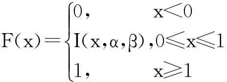
(4)

And

(5)

3BKNNSVM Algorithm

Combing with the analysis of KNNSVM algorithm and the features of the Beta distribution, we propose the BKNNSVM algorithm based on uncertainty calculation. The algorithm BKNNSVM improves the efficiency of the KNNSVM through controlling the amounts of KNN and LSVM classifiers.

3.1Uncertainty calculation of unlabeled samples based on Beta distribution

For binary classification problems, we can obtain the probability that each unlabeled sample belongs to positive class by Beta distribution when the neighbors′ distribution of the sample in the training dataset have known. Moreover, according to the features of Beta distribution, these samples′ probability which belong to the negative also meets the Beta distribution. Therefore, assuming an unlabeled samplexihasKneighbors in the training dataset which includem1positive samples andm2negative samples. The probability distribution whichxibelongs to the positive class is meets as (6).

Pr～Beta(α+1,β+1).

(6)

For different unlabeled samples, the probability which belong to positive class are also different. If the probability calculated by the Beta distribution is greater than 0.5, the positive class is the class which this unlabeled sample belongs. As a result, the value of t in (3) is 0.5. According to (3) and (5), the probability can be calculated as (7).

阿克苏诺贝尔的粉末涂料在不额外添加光源的情况下，就能让室内变得更加明亮，这将有助于改善与强化商业室内设计。

(7)

Due to the sum of probability from positive and negative is 1 for each unlabeled sample, the calculated probability of an unlabeled sample belongs to positive class which is closer to 0.5 means the uncertainty is greater. To obtain different uncertainty of each unlabeled sample, we define formula (8) to calculate uncertainty as below.

xi-uncertainty=min{I0.5(α+β),1-I0.5(α,β)}.

(8)

Andαmeans the amount of positive samples andβmeans negative samples of the neighbors for an unlabeled sample in the training dataset.

3.2BKNNSVM algorithm description

On the basis of above analysis, a method can be applied to decrease time consuming of the KNNSVM through reducing the amount of LSVM classifiers during the procedure of classification. Thinking about uncertainty calculation for each unlabeled sample, we propose the BKNNSVM algorithm to relax the strict limits of KNNSVM for increasing amounts of unlabeled samples which can be directly classified by KNN. That is to say, through calculating uncertainty of each unlabeled sample, only those samples with higher uncertainty need to build LSVM to further obtain their labels and labels of samples with lower uncertainty can be determined directly through KNN.

How to judge which samples′ uncertainty are greater? It is necessary to discover a thresholdUTand with thisUT, label of an unlabeled samplexiis obtained as formula (9). When the uncertainty ofxiis less thanUT, the label ofxiis obtained only through KNN, otherwise, a LSVM classifier should be built to further determine the label ofxi. We can control the time consumption through adjusting the value ofUT.

(9)

yrx(j)∈{-1,+1} means the label of thej-th nearest neighbor forxi.

TheKnearest neighbors is selected as formula (10).

(10)

The formula (10) has sorted all theKnearest neighbors.xrxi(1) is the nearest training sample andxrxi(j) is thej-th nearest one in the kernel space for an unlabeled samplexi.

The algorithm of BKNNSVM is described as bellow:

(2) Calculatingxi-uncertaintyofx′ through Beta distribution. Whenxi-uncertaintyis less than the thresholdUT, the label ofx′ is obtained only through KNN classifier and go to step (4). Otherwise go to step (3).

(3) Building a LSVM classifier forx′ by using itsKnearest neighbors to acquire the label ofx′. And go to next step.

(4) Go to the first step for estimating the label of the next unlabeled sample in the test dataset.

4Experiments and experimental results

To verify the performance of BKNNSVM, we compare the results of BKNNSVM and KNNSVM and KNN.

4.1Experimental data

We choose the four actual high-resolution remote sensing images with the resolution is 1 m from QUICKBIRD as shown in Fig. 1. They are all binary classification problems and the features of the four images are shown in Tab.1.

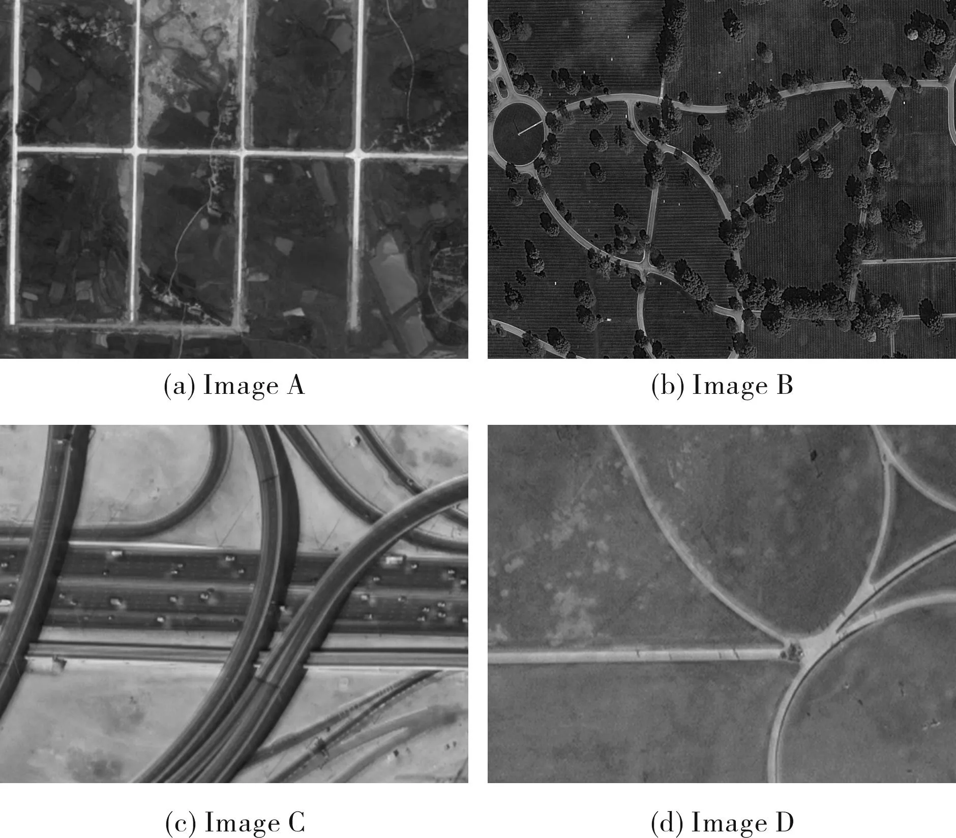
Fig.1　Four remote sense images图1　四幅遥感图像

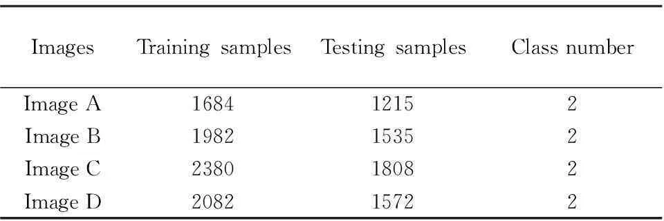
ImagesTrainingsamplesTestingsamplesClassnumberImageA168412152ImageB198215352ImageC238018082ImageD208215722

4.2Experiments

As mentioned above, the four images are classified with KNN, KNNSVM and BKNNSVM separately and all kernel functions used in the KNNSVM and BKNNSVM is RBF. For BKNNSVM, the thresholdUTis from 0 to 0.5, and increases 0.1 in each iteration. Meanwhile, we set upKfrom 5 to 95, and add 10 in each iteration. The contents of experiments are shown as bellow.

(1) The classification of sample proportion: the experiment tests the proportion change of samples classified through KNN and LSVM with algorithm BKNNSVM when theUTare different.

(2) The time consumption: the experiment verifies different time consumption under different thresholdUTwith BKNNSVM.

(3) The accuracy of classification: the experiment compares different classification accuracy with algorithms KNN, KNNSVM and BKNNSVM.

4.3Experimental Results

Based on above experimental contents, detailed experimental results have acquired shown as following.

4.3.1The change tendency of the classified samples′

proportion

Fig.2　The sample proportion classified by KNN under different threshold UT 图2　BKNNSVM在不同阈值下KNN分类样本数比例变化

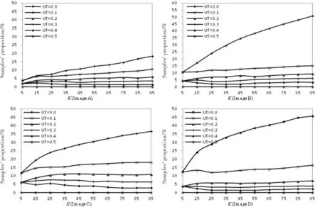
Fig.3　The sample proportion classified by LSVM under different threshold UT 图3　BKNNSVM在不同阈值下LSVM分类样本数比例变化

The curves shown in Fig. 2 and Fig. 3 are the tendency of samples′ proportion which calculated from the amount of samples through KNN and LSVM separately with different thresholdUTand neighbor′s numberK. The horizontal ordinate shows the value ofKand the ordinate denotes samples′ proportion of KNN and LSVM. Moreover, different curves denote differentUT. From Fig. 2 and Fig. 3, we can draw some conclusions. (1) The amount of samples classified through KNN algorithm directly decreases with the thresholdUTbecomes smaller. Especially, when theUTis very small, such as 0 or 0.1, the slope of the curve becomes larger which denotes the amount of samples classified through KNN decreases greatly. That is to say, samples classified through LSVM become more withUTis decreasing. All these results are shown that uncertainty of the unlabeled sample determines whether LSVM classifier should be built when the thresholdUTis certain.

(2) With the increasing of neighbors′ amountK, the number of samples classified through KNN directly becomes less and through LSVM is more and more. Because the value ofKis larger, the uncertainty of an unlabeled sample is also larger which leads to more LSVM classifiers should be built for further determining label for the samples.

4.3.2Time consumption with BKNNSVM

We verify the change tendency of time consumption with differentKand thresholdUTbased on BKNNSVM algorithm. As shown in Fig. 4, the horizontal ordinate shows the value ofKand the ordinate denotes time consumption metered with milliseconds. As the same as the first experiment, different curves denote differentUT. From Fig. 4, some results are obtained as following.

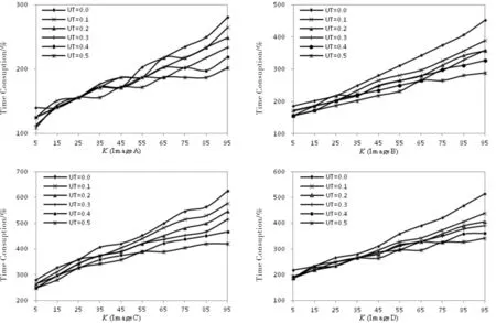
Fig.4　The tendency of time consumption of BKNNSVM with different threshold图4　BKNNSVM在不同阈值下运行时间变化趋势

(1) With the number ofKbecomes larger, the time consumption of the BKNNSVM increases more. This tendency can be explanted from two reasons, the first is the time consumption of searing neighbors for an unlabeled samplexiincrease with the number ofKbecomes larger; and the second is that when the number ofKis large, the uncertainty of an unlabeled sample also improves so that the amount of LSVM classifier becomes more. As a result, the time consumption becomes more withKincreases. (2) The time consumption decreases when the thresholdUTis larger, for the sake that the LSVM classifiers needed is less when theUTimproves. At the same time, when the number ofKis smaller, (such asK<45),UThas less impact on time consumption. Only when theKis larger, the impact becomes obviously. On the other hand, whenUTis smaller,Khas greater impact on time consumption and with theUTbecomes more, the impact decreases.

4.3.3The accuracy of Algorithm BKNNSVM

The accuracy tendency of classification on BKNNSVM withKand threshold are also tested and the results are shown as Fig.5. The accuracy is defined as correct rate which is the radio of correct classified samples and all the samples in the test dataset. From the Fig. 6, we can draw conclusions as follow.

(1) When theUTbecomes more and more, the accuracy of the algorithm BKNNSVM decreases. For the sake that whenUTis more, the number of samples which are classified by KNN directly is greater and the LSVM classifiers needed is less. As a result, the accuracy becomes descendant. Especially, whileUTequals 0.5, all the samples in the test dataset are classified by KNN which leads to the minimum accuracy. Meanwhile, from the four images, whenUTis smaller, the accuracy is higher. Specially, the two curves whenUTequals 0.0 and 0.1, the accuracy of the algorithm are the similar, even in the image D, the curve withUTequals 0.1 is higher thanUTequals 0. All these are shown, when theUTis very smaller, the accuracy of BKNNSVM are similar.

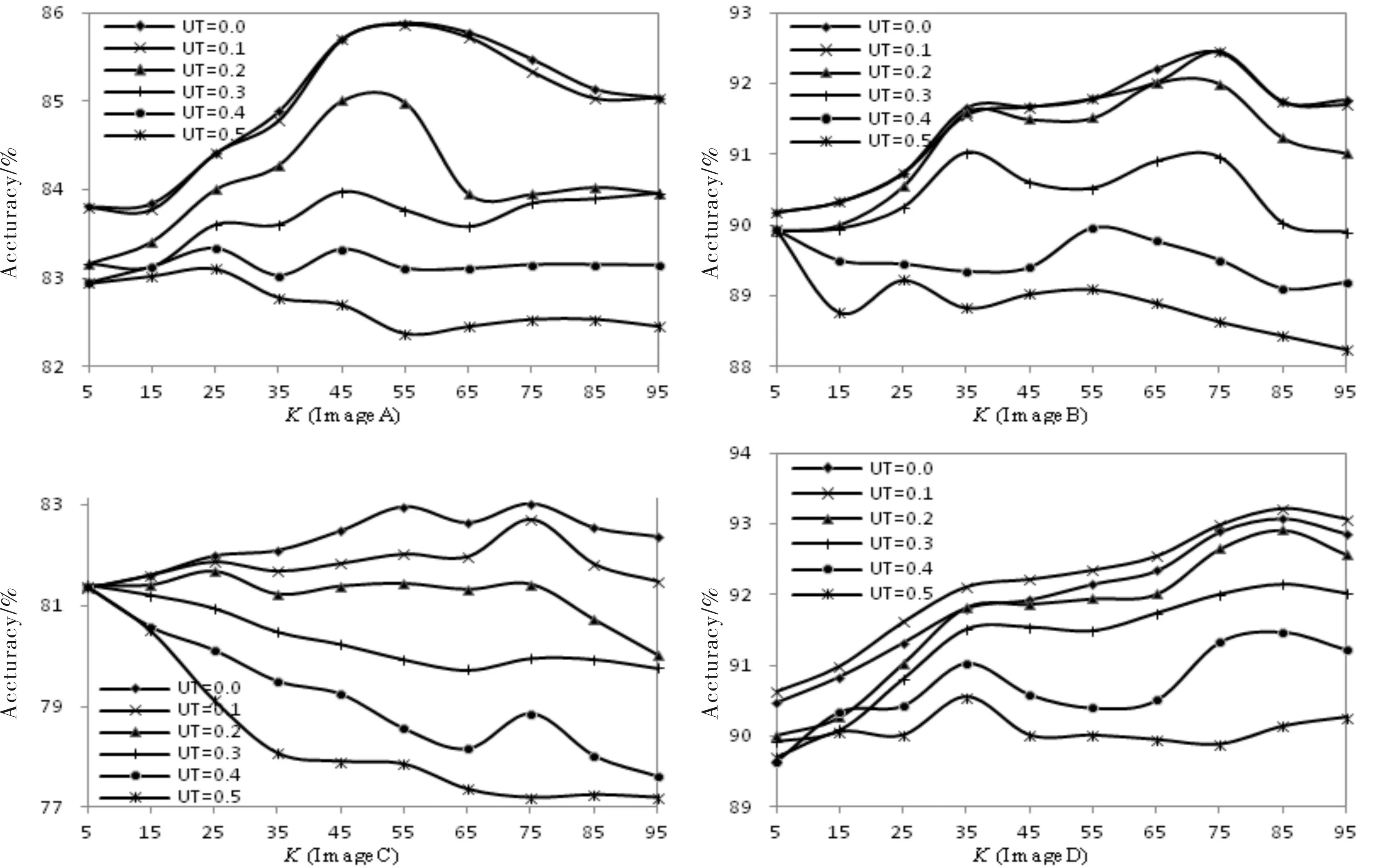
Fig.5　The accuracy of BKNNSVM with different threshold图5　不同阈值下BKNNSVM的精度变化曲线

(2) When theKbecomes more and more, the curves of accuracy shows the tendency of increases gradually at first, and then decreases. For KNN algorithm, the similarity of theKnearest neighbors and the unlabeled samples are very great which brings about more accuracy classified results. And on the other hand, with the sameUT, more LSVM classifiers should be built with smallerKwhich leads to less accuracy. With these two factors, when theKis more and more from 0, the increased accuracy from LSVM is larger than decreased accuracy from KNN, the accuracy of the algorithm improves; while improves to a certain number, KNN classifier has more impact on the whole accuracy of BKNNSVM, consequently, the whole accuracy curve is descendent. Especially, when theKis more, the local feature of the LSVM has been broken and the accuracy of KNN and LSVM both decrease. 4.3.4Comprehensive analysis of all the experimental

results

Combing of Fig.2,Fig.3,Fig.4 and Fig.5,whenUTequals 0, the results from BKNNSVM is the results from KNNSVM; and whenUTequals 0.5, the results comes from KNN directly. Synthesizing all the results of the above experiments, we can draw conclusions as below.

For time consumption, the algorithm BKNNSVM is between the algorithms KNNSVM and KNN. Especially, whenKis larger, the effect of decreasing time consumption is obvious; and at the same time, the accuracy is similar or even higher than KNNSVM withUTis from 0 to 0.1. This explains that the algorithm BKNNSVM can reduce time consumption effectively and retain the similar accuracy as algorithm KNNSVM among this threshold range. Although with the increasing amount of threshold, the accuracy of BKNNSVM becomes lower and the time consumption decreases very obviously. Consequently, BKNNSVM has ability to further optimize KNNSVM on the basis of the balance of time cost and accuracy with reasonable threshold.

5Conclusions

Due to the high resolution remote sensing images have a massive amount of data, in order to improve the efficiency of these images′ classification, the paper proposes algorithm BKNNSVM which is based on uncertainty calculation of unlabeled samples to further optimize the algorithm KNNSVM. For binary problem, the distribution of unlabeled samples are satisfied for Binomial distribution so that probabilities of these unlabeled samples belong to positive or negative class are satisfied to Beta distribution. With Beta distribution, each unlabeled sample′s uncertainty may be calculated and compared with threshold. If the uncertainty of the unlabeled sample is lower than threshold, the KNN classifier is applied for classification directly and LSVM is built for classification when the uncertainty is more than threshold. The experimental results show that compared with KNNSVM, BKNNSVM has powerful ability to reduce time consumption and retain similar classified accuracy with appropriate threshold. Consequently, BKNNSVM is a kind of algorithm which is fit to deal with the high resolution remote sensing images.

Acknowledgement

The project was supported by the National Nature Science Foundation of Hubei Province (PBZY14019)for the financial assistance.

References

[1]Yinhui Zhang, Gengxing Zhao. Reviews of land use / land cover classification methods of Remote Sensing Research [J]. Chinese Journal of Agriculture Resources and Regional Planning, 2002, 23(3): 21-25.

[2]Ke C, Bao-ming Z, Ming-xia X. Based on fuzzy Bayes decision rules change detection approach of remote sensing images[C]//IEEE. Urban Remote Sensng Evnt, 2009 Joint. New Jersey: IEEE, 2009: 1-6.

[3]Xie X, Zhao J, Li H, et al. A SPA-based K-means clustering algorithm for the remote sensing information extraction[C]//IEEE. Geoscience and Remote Sensing Symposium (IGARSS), 2012 IEEE International. New Jersey: IEEE, 2012: 6111-6114.

[4]Hongmei Zhang, Jiwen Wu, Xing Liu, etc. Feature extraction and decision tree classification of land use remote sensing images [J]. Science of Surveying and Mapping, 2014, 39(010): 53-56.

[5]Vapnik V. The nature of statistical learning theory [M]. Berlin: Springer, 2000.

[6]Xiaoming Wang, Mengqi Mao, Changjing Zhang, et al. A comparative study of remote sensing image classification based on support vector machine [J]. Geomatics & Spatial Information Technology, 2013 (4): 17-20.

[7]Camps-Valls G, Mooij J, Schölkopf B. Remote sensing feature selection by kernel dependence measures [J]. Geoscience and Remote Sensing Letters, IEEE, 2010, 7(3): 587-591.

[8]Liheng Fan, Junwei Lv, Zhentao Yu, et al. Classification of hyperspectral remote sensing images with fusion multi spectral features based on kernel mapping [J]. Acta Photonica Sinica, 2014, 43(6): 630001-630006.

[9]Brailovsky V L, Barzilay O, Shahave R. On global, local, mixed and neighborhood kernels for support vector machines [J]. Pattern Recognition Letters, 1999, 20(11): 1183-1190.

[10]Zhang H, Berg A C, Maire M, et al. SVM-KNN: Discriminative nearest neighbor classification for visual category recognition [C]//IEEE. Computer Vision and Pattern Recognition, 2006 IEEE Computer Society Conference on. New Jersey: IEEE, 2006, 2: 2126-2136.

[11]Blanzieri E, Melgani F. Nearest neighbor classification of remote sensing images with the maximal margin principle [J]. Geoscience and Remote Sensing, IEEE Transactions on, 2008, 46(6): 1804-1811.

[12]Cheng H, Tan P N, Jin R. Efficient algorithm for localized support vector machine [J]. Knowledge and Data Engineering, IEEE Transactions on, 2010, 22(4): 537-549.

[13]Segata N, Blanzieri E. Fast and scalable local kernel machines [J]. The Journal of Machine Learning Research, 2010, 11: 1883-1926.

[14]L GyNorfi. On the rate of convergence of nearest neighbor rules [J]. IEEE Transactions on Information Theory, 29:509-512, 1978.

[15]Mudd, Grey Bill, Ding Hua. Introduction to statistics [M]. Beijing: Science Press, 1978.

基于BKNNSVM算法的高分辨率遥感图像分类研究

舒振宇1，周城1，王典洪2

(1中南民族大学 电信学院，武汉430074； 2中国地质大学 地球物理与空间信息学院，武汉430074)

摘要为了解决局部支持向量机算法KNNSVM存在的分类时间过长不利于具有海量数据量的高分辨率遥感图像分类的不足，提高KNNSVM的算法表现，提出了改进的基于不确定性的BKNNSVM算法.该算法利用二项式分布的共轭先验分布Beta分布根据近邻的分布情况推导该未标记样本属于正类或负类的概率大小，从而计算每一个未标记样本在类属性上的不确定性大小.再通过设置不确定性阈值的大小，对不确定性低于阈值的未标记样本直接采用KNN进行分类，而对高于阈值的样本利用其近邻建立局部支持向量机分类器进行分类.对高分辨率图像分类的实验结果表明:合适的阈值能够有效降低原始KNNSVM算法的时间开销，同时能保持KNNSVM分类精度高的特点.

关键词高分辨率遥感图像分类;KNNSVM算法;BKNNSVM算法

中图分类号TP39

文献标识码A

文章编号1672-4321(2016)01-0095-08

基金项目湖北省自然科学基金资助项目(PBZY14019)

作者简介舒振宇(1978-)，男，讲师，博士，研究方向：图像分类，E-mail：zhenyushu@scuec.edu.cn

收稿日期2016-01-20