ARTICLE Hermiticity of Hamiltonian Matrix using the Fourier Basis Sets in Bond-Bond-Angle and Radau Coordinates†
2016-04-08DequnYuHeHungGunnrNymnZhigngSunStteKeyLbortoryofMoleulrRetionDynmisndCenterforTheoretilndComputtionlChemistryDlinInstituteofChemilPhysisChineseAdemyofSieneDlin116023ChinbShoolofPhysisndEletroniTehnologyLioningNor
De-qun Yu,He Hung,b,Gunnr Nymn,Zhi-gng Sun,d∗.Stte Key Lbortory of Moleulr Retion Dynmis nd Center for Theoretil nd Computtionl Chemistry,Dlin Institute of Chemil Physis,Chinese Ademy of Siene,Dlin 116023, Chinb.Shool of Physis nd Eletroni Tehnology,Lioning Norml University,Dlin 116029,Chin.Deprtment of Chemistry,Physil Chemistry,G¨oteborg University,SE-412 96 G¨oteborg,Swedend.Center for Advned Chemil Physis nd 2011 Frontier Center for Quntum Siene nd Tehnology,University of Siene nd Tehnology of Chin,Hefei 230026,Chin(Dted:Reeived on July 4,2015;Aepted on July 13,2015)
ARTICLE Hermiticity of Hamiltonian Matrix using the Fourier Basis Sets in Bond-Bond-Angle and Radau Coordinates†
De-quan Yua,He Huanga,b,Gunnar Nymanc,Zhi-gang Suna,d∗
a.State Key Laboratory of Molecular Reaction Dynamics and Center for Theoretical and Computational Chemistry,Dalian Institute of Chemical Physics,Chinese Academy of Science,Dalian 116023, China
b.School of Physics and Electronic Technology,Liaoning Normal University,Dalian 116029,China
c.Department of Chemistry,Physical Chemistry,G¨oteborg University,SE-412 96 G¨oteborg,Sweden
d.Center for Advanced Chemical Physics and 2011 Frontier Center for Quantum Science and Technology,University of Science and Technology of China,Hefei 230026,China
(Dated:Received on July 4,2015;Accepted on July 13,2015)
In quantum calculations a transformed Hamiltonian is often used to avoid singularities in a certain basis set or to reduce computation time.We demonstrate for the Fourier basis set that the Hamiltonian can not be arbitrarily transformed.Otherwise,the Hamiltonian matrix becomes non-hermitian,which may lead to numerical problems.Methods for correctly constructing the Hamiltonian operators are discussed.Speci fi c examples involving the Fourier basis functions for a triatomic molecular Hamiltonian(J=0)in bond-bond angle and Radau coordinates are presented.For illustration,absorption spectra are calculated for the OClO molecule using the time-dependent wavepacket method.Numerical results indicate that the non-hermiticity of the Hamiltonian matrix may also result from integration errors. The conclusion drawn here is generally useful for quantum calculation using basis expansion method using quadrature scheme.
Key words:Discrete variable representation,Hermiticity,Time-dependent wavepacket method,Absorption spectra
†Part of the special issue for“the Chinese Chemical Society’s 14th National Chemical Dynamics Symposium”.
∗Author to whom correspondence should be addressed.E-mail: zsun@dicp.ac.cn
I.INTRODUCTION
Quantumdynamicscalculationswithmolecular Hamiltonians have witnessed enormous progress.In the past years,a number of numerical techniques have been proposed to reduce the integration time for constructing the Hamiltonian matrix for a chosen basis set and to improve the accuracy of the numerical results[1–12].This makes it possible to accurately simulate complex molecular dynamics and to calculate ro-vibrational spectra[13–19].However,exact quantum calculations beyond triatomic and tetra-atomic molecules are still a formidable task.Improving the computational methods will be of continued interest in the theoretical fi eld.
Quantum dynamics calculations solving the timedependent molecular Schr¨odinger equation have proven to be invaluable for understanding dynamical process like photodissociation and femtosecond real-time experiments[20–22].In an accurate triatomic molecular calculation,the Hamiltonian used is often described in Jacobi[23],Radau[24,25],hyperspherical[26,27],or bond-bond angle coordinates[25,28].Fourier series or particle-in-the-box eigenfunctions are commonly used to expand the nuclear wavefunction along the radial degrees of freedom.As to the angular degree(s)of freedom,usually spherical harmonics(Legendre polynomials)basis functions are used.The numerical results of such calculations have been shown to be of exponential convergence[9,29].
The standard fast-Fourier transform(FFT)technique can be directly applied to propagate the initial wavepacket when the Fourier series are used as basis functions[29].The introduction of the FFT[30,31] technique led a surge of time-dependent wavepacket applications.The FFT technique is easy to implement, even for complex kinetical operators[28].At the same time,the obtained physical concept is clear,similar to that in a time-dependent classic dynamics.
Several time-dependent wavepacket calculations have illustrated that the Fourier functions can also be used as the basis set for the angular variable(s)[28,32–41]. However,using the Fourier basis functions for the angular variable(s),singularities may be encountered.Several groups have investigated this problem and proposed to use a transformed Hamiltonian or to use cosθ instead of θ as the angular variable to avoid the di ffi culty withsingularities[28,32–37,39].Moreover,to propagate the wavepacket with the convenient second order split operator method,which is combined with the FFT technique,a transformation of the triatomic Hamiltonian may be required[24,26,42].
In this work,we point out that once a set of orthogonal basis functions have been chosen,for instance the Fourier basis set,there are limitations on how the Hamiltonians may be transformed.Otherwise the Hamiltonian matrix may become non-hermitian,leading to numerical problems.Tuvi et al.[43]have investigated the non-hermiticity problem using the Fourier grid Hamiltonian(FGH)discrete variable representation(DVR)method[39].They suggested that to improve the numerical convergence,the Hamiltonian operators should be in explicitly symmetric form.If the Fourier basis set is chosen,the Hamiltonian should be kept in an explicitly symmetric form to avoid nonhermiticity resulting from integration errors.
In the following we will explicitly consider timedependent wavepacket calculations using the Fourier basis sets and various triatomic Hamiltonians in bond bond-angle and Radau coordinates.The A2A1←X2B1absorption spectrum of the OClO molecule is calculated to illustrate the e ff ect of transforming the Hamiltonian or changing the form of the Fourier basis set to the numerical results.Two types of non-hermiticity will be considered.The fi rst type we will refer to as analytical non-hermitcity.It results from the use of a Hamiltonian and basis set in which the Hamiltonian matrix is non-hermitian even if it can be analytically constructed.The second type we will refer to as numerical non-hermiticity where the non-hermiticity in the Hamiltonian matrix results purely from integration errors.
In this work,we discuss normalization of the wavefunction,review the principles of the FFT technique and discuss how non-hermiticity arises in the Hamiltonian matrix in a Fourier basis set representation. Hamiltonians for triatomic molecules in bond bond angle and Radau coordinates are used for illustration. Numerical illustrations of the issues discussed are presented.This is done by calculating the absorption spectrum of the OClO molecule with a 3D(J=0)timedependent wavepacket model in Eckart and Radau coordinates.
II.KINETIC ENERGY OPERATORS,THEIR EVALUATION AND HERMITICITYA.Kinetic energy operators and wavefunction normalization
The Hamiltonian of the system can be expressed as a sum of the kinetic energy operator(ˆT)and the potential energy surface(V)in the nonrelativistic limit and
within the Born-Oppenheimer(BO)approximation,

Starting with the Lagrangian form of the kinetic energy in terms of classic velocities,successive transformations lead to
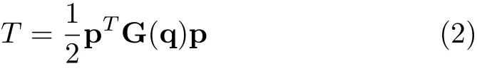
where piis the momenta conjugate to the chosen coordinates qi(linearly independent),and G(q)is the wellknown G matrix

where xidenotes the Cartesian coordinates of atom i with a mass of mi.Then,the Podolsky formalism[44] yields the quantum mechanical operator
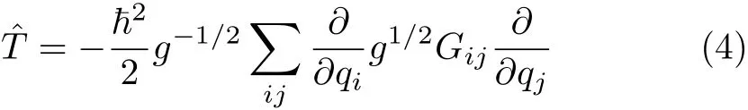
where g=|g|=|G−1|is the determinant of the metric tensor matrix g[45].The operator in Eq.(4)gives the normalization of the wavefunction Ψ(q)as
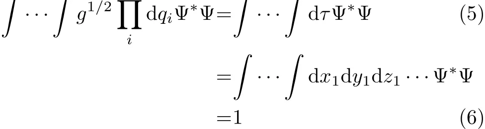
However this standard normalization of Ψ with the weight factor g1/2(normalized with volume element dτ=dx1dy1dz1···in cartesian coordinates[46]),is not always used.Podolsky[44]considered a transformed wavefunction normalized with the weight factor equal to 1,that is
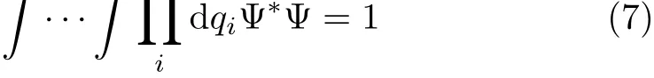
with the kinetical operators being
Let us assume that the determinant g(q)can be represented as a product of two independent factors g(q)=gA(qA)gB(qB)where q=(qA,qB)and let us transform the wavefunction Ψ(q)to

which,following from Eq.(5),ful fi lls the normalization condition:
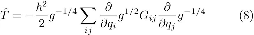
For gA=1 and gB=g this equation gives the standard normalization de fi ned by Eq.(5),and for gA=g and gB=1 it gives the normalization with weight factor unity,which Podolsky considered[44].Because the factoris associated with the transformation of the wavefunction,we will refer toas the transformation factor in order to distinguish from the weight factor.We note here that,if the weight factoris equal to 1(that is,with transformation factor as g), the operators can always be rearranged in an explicitly symmetric form[8,44],as shown in Eq.(8).
Let us categorise triatomic Hamiltonians in bondbond angle coordinates that have appeared in the literature according to the associated transformationand weightfactors[16].The HamiltonianHˆwconsidered by for instance Bardo and Wolfberg[47,48] falls in the category of Podolsky’s normalization(weight factorequal to 1)[16].The Hamiltonian can be written[47,48],
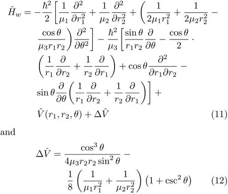
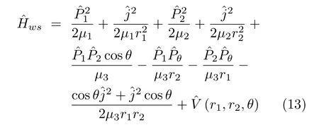
whereµ1,µ2,andµ3are the related(reduced)masses. The other variables have their traditional de fi nitions. As we have noted,since this HamiltonianˆHwhas a corresponding weight factor of unity and transformation factor g,it can be rearranged into an explicitly symmetric form
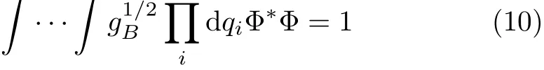
This Hamiltonian gives the wavefunction normalization condition[16,47,48]

The HamiltoniansˆHwandˆHwsare not generally used. However,the HamiltonianˆHcin bond bond angle coordinates given by Carter and Handy[49]is more often used,
大樱桃不宜在过分寒冷的地区发展。冬季来临之际,应对幼树采取树干培土、缠膜、涂白等措施以防止冻害发生。休眠期修剪一般在发芽前进行,避免剪口在寒冷的冬季失水,冻伤树体。
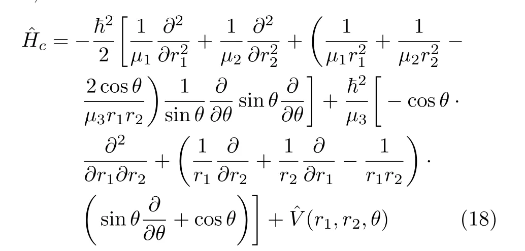
A rearranged formˆHcaof this Hamiltonian is
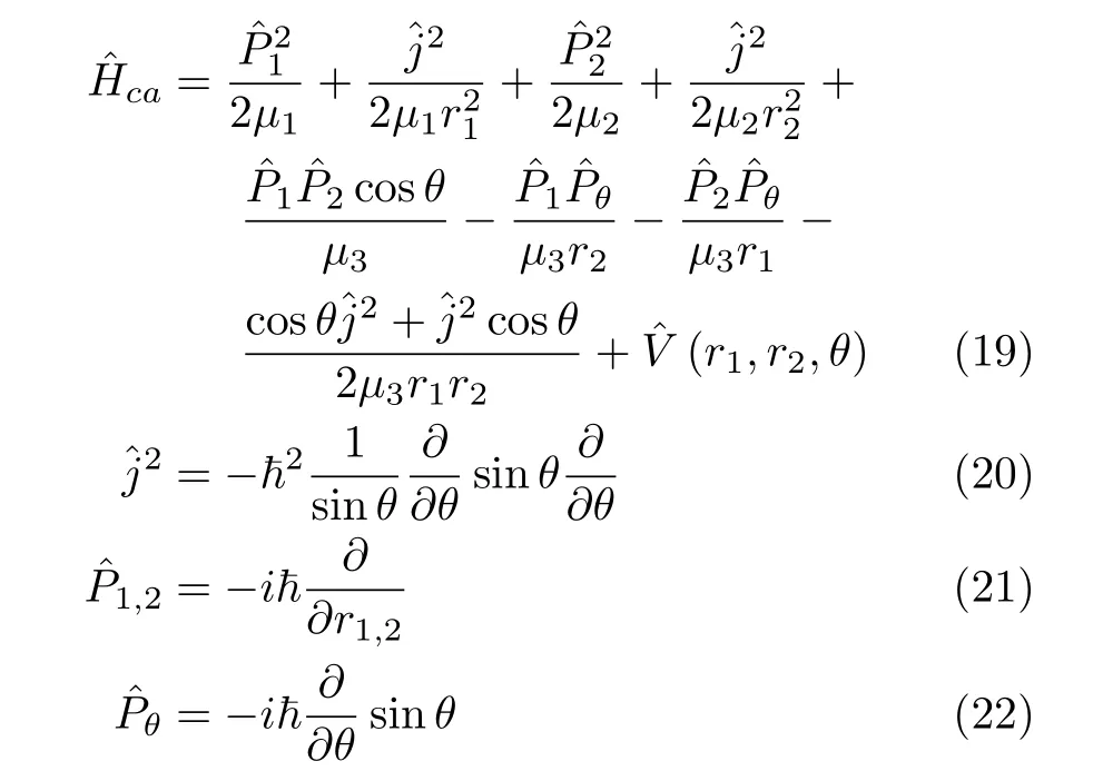
The latter Hamiltonian gives the wavefunction normalization[49],
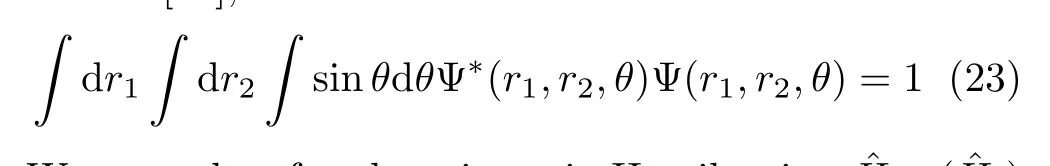
We note that for the triatomic HamiltonianˆHca(ˆHc) in bond-bond angle coordinates,the weight factor
g1/2B=sinθ.Therefore,the operators ofˆHccannot be written into an explicitly symmetric form.
B.Action of the kinetic energy operator using Fourier transform
In a time-dependent quantum calculation,the action of the potential operators on the wavefunction is sim-ple multiplication when a spatial representation is used. The evaluation of the action of the kinetic energy operator will be in this representation however involve derivatives of the wavefunction.The derivatives can be e ffi ciently found by the Fourier transform technique, which transforms to momentum space where the kinetic energy operator is local and only multiplication with the wavefunction is required.
The forward Fourier transformFT(x,k)is de fi ned as
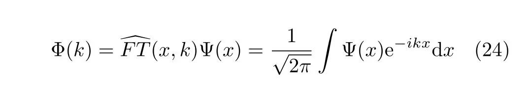
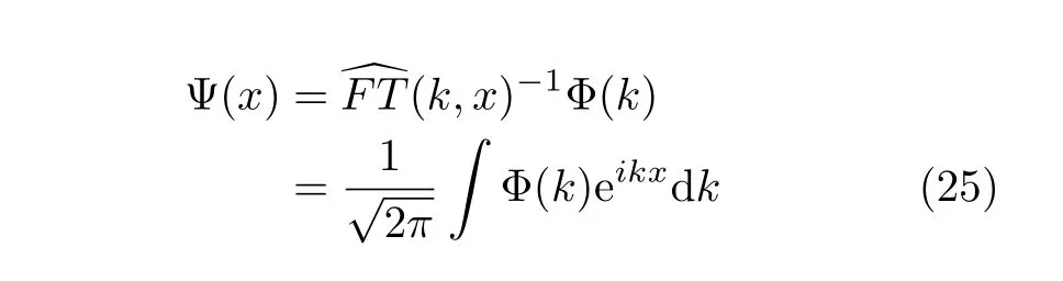
It transforms the wavefunction from the space representation to the momentum representation.Similarly to Eq.(24),the backward Fourier transformFT(x,k)−1 is given byd
It is easy to see that for the derivatives of the wavefunction we can write

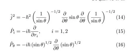
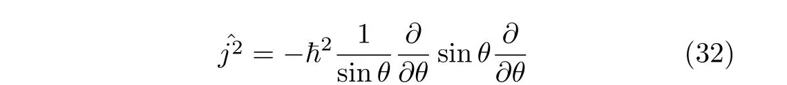
Thus the derivatives are evaluated as simple multiplications in the momentum space.Treating complicated kinetic operators with Fourier transform can be derived straightforwardly.For instance,the action of the opera-(this is the angular momentum operator which is used in the later sections,see Eq.(42)) on the wavefunction can be written as


We note here that when model Hamiltonian is expressed in a suitable form,such as the HamiltonianˆHcaand ˆHws,the action of each kinetic operator on the wavefunction always consists of a combination of two fi rst derivatives.As a result,the factor i(imaginary unit) resulting from a single evaluation of the fi rst derivative using the Fourier transform technique does not appear in the numerical implementation.
C.Hermiticity of the angular momentum operator using the Fourier basis
1.Hermiticity
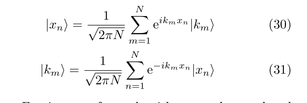
Propagating the wavepacket using Fourier transform in a time-dependent calculation is principally equivalent to evolving the wavefunction using a Fourier series.In the numerical calculation,the spatial and momentum coordinates have to be discretized as|xn>and |km>which enables the implementation of the FFT technique.The transformation between the discrete spatial coordinate representation|xn>and the discrete momentum representation|km>is given by
Fast Fourier transform algorithms can be employed to a ff ect these transformations and to compute derivative(s)of the wavefunction for realizing the action of the operator on the wavefunction or the wavefunction multiplied by functions of the spatial coordinates.In order to have a good representation of the system,the Hamiltonian matrix should be hermitian in the discrete Fourier space.Tuvi et al.[43]have shown that writing operators of a one-dimensional nuclear Hamiltonian in an explicitly symmetric form guarantees the hermiticity of the resulting Hamiltonian matrix.Their conclusion can be extended directly to multi-dimensional problems.Therefore the Hamiltonian operators given by the Podolsky normalization condition[44]are de finitely hermitian in a Fourier basis set.We may use the corresponding Hamiltonian form,that is,use Hamiltonian with weight factor=1 in our calculation using a Fourier basis set.
A transformationcan be made to remove the weight factor sinθ−1/2.The transformed operator then becomes
This means that we write the angular momentum operator using Podolsky’s normalization condition[44]and the weight factor gBbecomes unity[16].Hence the operator is de fi nitely symmetric.For a triatomic case,this corresponds to transforming the Hamiltonian fromˆHcain Eq.(19)toˆHwsin Eq.(13).When the Fourier basis set 1/√
2πNe−iknθis used in a calculation where the angular momentum operator in Eq.(34)is employed, problems with non-hermiticity do not arise.
2πNe−iknCin the calculation,whereby the resulting Hamiltonian matrix becomes hermitian.In this way the triatomic Hamiltonian can be obtained in an explicitly symmetric from.From the discussion above,it is clear that to decide whether an operator,particularly the Hamiltonian operator,is hermitian or not,the basis set has to fi rst be decided.
2.Integration error
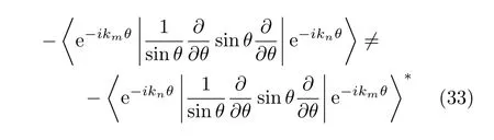
Considering the integration error,the Hamiltonian operators used in the numerical calculation should be in an explicitly symmetrical form when the discrete Fourier basis is used[43].Sometimes although a Hamiltonian operator is theoretically hermitian in some basis set,the resulting Hamiltonian matrix becomes nonhermitian in the numerical calculations.For instance, the operator in Eq.(35)andare equivalent and hermitian in a Fourier basis set when the integration is exact.However because of the integration errors resulting from the discretization,the operator in Eq.(37)is not numerically hermitian in the discrete Fourier basis set.This is because the correspo
and its hermitian conjugate,
are only equivalent if there is an odd number of grid points N and m=l[43],where Ci=i∆C,i=1,...,N. Thus[43],when the model Hamiltonian used in an FFT time-dependent calculatition contain operators of the form in Eq.(37),the numerical results may be unreliable.
D.Hermiticity of the J=0 triatomic Hamiltonian in
bond-bond angle and Radau coordinates in the Fourier basis
The commonly used triatomic Hamiltonian(J=0) in bond-bond angle coordinates(r1,r2,θ)written in the form ofˆHpswith weight factor gBequal to 1 is explicitly symmetric.Therefore the resulting Hamiltonian matrix is hermitian[43]in the Fourier basis setbelow referred to as FBST.However,the rearranged formˆHof the Hamiltonian in Eq.(18),with weight factor given by Carter and Handy[49] does not lead to a hermitian matrix using the FBST basis set and is not suitable for an FFT calculation.As we have discussed,the transformation factor can either be absorbed by a transformation of the Hamiltonian sinθ1/2ˆHsinθ1/2or by changing the variable θ to cosθ.From the work of Carter and Handy[49],the HamiltonianˆHcsin bond-bond angle coordinates, taking r1,r2and C=cosθ as the variables,can be written as,

The operators of this Hamiltonian are in explicitly symmetric form and result in a herm√itian matrix with the Fourier basis set(FBSC):{1/2πNe−iklr1,
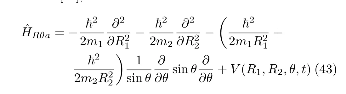
Similar conclusions hold for the Hamiltonian in Radau coordinates.The usually used Hamiltonian (J=0)in Radau coordinates(R1,R2,θ),can be written as[50], where m1and m2are the relevant masses.Note that the variable θ here has a di ff erent meaning from that in bond bond-angle coordinates.This Hamiltonian has a volume element α−3sinθdR1dR2dθ where,with weight factorequal to sinθ−1/2.Its resulted Hamiltonian matrix is not hermitian in the FBST basis set due to the transformation factor sinθ−1/2.Similar to the case in bond-bond angle coordinates,the Hamiltonian in Eq.(43)can be rewritten as

The di ffi culty arising from the transformation factor1/√
sinθhasbeeneliminatedwhentaking (R1,R2,cosθ)as the variables instead of(R1,R2,θ)and using the FBSC basis set.The Hamiltonian operator is now explicitly symmetric and the resulting Hamiltonian matrix is hermitian.
The Hamiltonian in Radau coordinates can also be transformed[24,42]
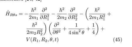
with the weight factor being equal to 1.Therefore,the HamiltonianˆHRθsresults in a hermitian matrix in the FBST basis set.The Hamiltonian has a volume element dR1dR2dθ.
We can expect that the convergence of the calculations are good using the HamiltonianˆHwsin Eq.(13) orˆHRθsin Eq.(45)with the FBST basis set and using ˆHcsin Eq.(40)orˆHRcsEq.(44)with the FBSC basis set.However,calculations using the HamiltonianˆHcain Eq.(19)orˆHRθain Eq.(43)with either of the two Fourier basis sets should be only conditionally stable and exhibit numerical di ffi culties.
Sometimes the HamiltonianˆHwsin Eq.(13)is used in the expanded formˆHwin Eq.(11),or the Hamiltonian ˆHRcsin Eq.(45)is used in the form,
III.NUMERICAL EXAMPLES
In this section,we will show absorption spectra of the OClO molecule calculated with the time-dependent wavepacket method using Hamiltonians in bond-bond angle and Radau coordinates to illustrate the arguments put forwˆard above.Results oˆbtained using the HamiltonianHcsin Eq.(40)andHRcsin Eq.(44)using the FBSC basis set are comˆpared with results calˆculated using the HamiltonianHwsin Eq.(13)andHRθsin Eq.(45)using the FBST basis set.These comparisons are used to check the convergence of the calculation using the FFT technique.From the discussion above,we know that these four numerical models should exhibit the best convergence.ˆ
The results using the HamiltonianHcain Eq.(19)and Hˆwsin Eq.(13)with the FBST basis set are compared in order to investigate the non-hermiticity problem caused by the wˆeight factor.The calculations using the HamˆiltonianHwin Eq.(11)with the FBST basis set andHRin Eq.(46)with the FBSC basis set are carried out and compared with the results from the best converged models,in order to investigate the non-hermiticity pˆroblem cˆaused purely by integration errors when usingHwand HR.We fi nd that for the present application even for a short time propagation a non-hermitian Hamiltonian matrix may make the results unreliable.
OClO is a molecule of both experimental and theoretical interest,due to its presumed role in polar stratospheric ozone depletion.Accurate 3D ab initio nearequilibrium potential energy surfaces(PESs)of the X2B1ground state and the excited state,A2A2,have been reported[51].The PES of the A2A1state has a C2vequilibrium geometry and features strong coupling between the anti-symmetric and the symmetric stretch modes.The two surfaces reproduce the experimental absorption spectrum well[25]and these surfaces are used here.The equilibrium geometries of the both PESs are far from linear with deep bending wells,which enable us to ignore the singularity problem found for linear geometries[32–35].
The absorption spectrum of the OClO molecule is obtained by Fourier transforming the time autocorrelation function of the initial wavefunction.The initial ground vibrational eigenfunction of the X2B1electronic state is obtained by a variational calculation using Morse-Morse harmonic wavefunctions[26].We note that even though the method used for obtaining the initial wavefunction leads to a non-hermitian Hamiltonian matrix, its in fl uence on the quality of the ground wavefunction is marginal[24].The method has been detailed in our previous work[24–26].The absorption spectra below are uniformly broadened with a Lorentzian function of 20 cm−1FWHM(full width at half maximum) by damping the autocorrelation functions with an exponential function.In the following calculation,a Chebyshev propagator is applied to evolve the initial wavefunction on the excited PES.The round o ff error in the Chebyshev polynomial expansion is less than 1×10⁻¹⁵. Usually the time-step is chosen to be 0.7 fs and a total of 1024 time steps is enough to obtain a converged spectrum.
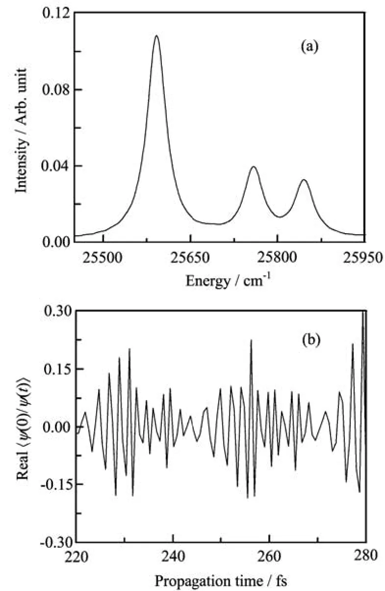
FIG.1(a)An expanded portion of the calculated absorption spectra and(b)the real part of the correlation functions <ϕ(0)|ϕ(t)>usingˆHwsin Eq.(13)with FBST(solid lines)and ˆHcsin Eq.(40)with FBSC(dotted lines).
A.In Eckart coordinates
1.Hermitian Hamiltonian matrix
The HamiltonianˆHwsin Eq.(13)using the Fourier basis set FBST results in a Hermitian matrix as does the HamiltonianˆHcsin Eq.(40)using FBSC since these Hamiltonians are in explicitly symmetric forms[43].We can expect that the results obtained with these two numerical models should agree with each other and show good numerical convergence.In the calculations with the HamiltonianˆHwswe set the grid ranges to[2.3,4.8] in atomic units for r1and r2and[1.3,2.7]in radians for θ.ForˆHcswe set the grid ranges[2.3,4.8]in atomic units for r1and r2and and[−0.9,0.25]for cosθ.For each calculation,64×64×32 grid points are used(64 grid points along each radial coordinate and 32 along the angular coordinate).Convergence concerning grid ranges and grid spacing has been checked.
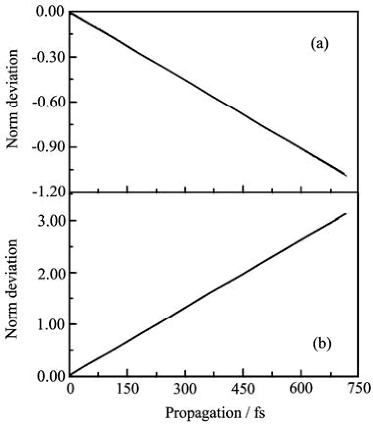
FIG.2Time-dependent norm deviation from its initial value 1 of the wavefunction usingˆHwsin Eq.(13)with FBST (a)andˆHcsin Eq.(40)with FBSC(b).
A typical part of the absorption spectra of the two numerical models is shown in Fig.1(a).The corresponding real part of the correlation functions are shown in Fig.1(b).The results are virtually identical for the two models,indicating good numerical convergel.The norm of the evolved wavepacket is not guaranteed to be conserved in a Chebyshev propagation and the timedependence of the norm gives a measure of convergence.The deviation of the norm from unity usingˆHwsin the FBST representation is shown in Fig.2(a),and that usingˆHcsin the FBSC representation is shown in Fig.2(b).We see that the norm is excellently conserved.
2.Non-hermitian Hamiltonian matrix
In this subsection,we only calculate the OClO absorption spectrum using the HamiltonianˆHcin Eq.(18) with the FBST basis set parameters used in subsection III(A).As we have discussed,the resulting Hamiltonian matrix is non-hermitian.Although the derivatives of the wavefunction can be evaluated accurately with FFT,the non-hermiticity of the Hamiltonian matrix makes the numerical results unreliable.The calculated absorption spectrum is shown in Fig.3(b)together with the exact result of Fig.1.There are a clear deviations.The heights of the peaks have been altered by the non-hermiticity of the Hamiltonian matrix,and a ghost peak has arisen.The time-dependent norm of the wavefunction is shown in Fig.3(a).We see drastical norm violation,which indicates that the non-hermitian matrix develops complex eigenvalues.Thus the numerical model is not stable.We note that the period of the initial oscillation of the time-dependent norm approximately agrees with that of the symmetric stretch of the
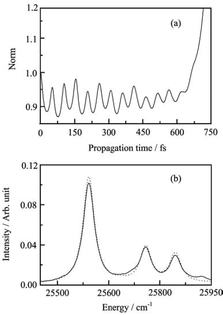
FIG.3(a)The time-dependent norm of the wavefunction resulting from using the non-hermitian matrix of the HamiltonianˆHcin Eq.(18)with FBST.(b)The solid line is the expanded portion of the calculated absorption spectra using the HamiltonianˆHcin Eq.(18)with FBST and the dotted line is the exact result shown in Fig.1.
3.Numerically non-hermitian Hamiltonian matrix
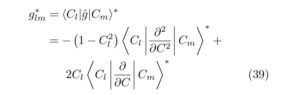
For numerical convenience,sometimes the expanded form in Eq.(11)of the HamiltonianˆHwsis used in numerical calculation.As Tuvi et al.pointed out[43],as long as the operators are not explicitly symmetric and the Fourier basis set is applied,the resulting Hamiltonian matrix becomes non-hermitian because of integration errors.The operators
in Eq.(11)make the Hamiltonian martix numerically non-hermitian.We may expect that this nonhermiticity resulting purely from integration errors should be less drastic than analytic non-hermiticity. However,although the spectrum is satisfactory,which indicates that the non-hermiticity of the Hamiltonian matrix only slightly in fl uences the numerical results, the norm of the wavefunction increases exponentially with propagation time,see Fig.4.This was not observed usingˆHwswith the FBST basis set.The timedependent norm is also sensitive to the values of theChebyshev parameters,which again indicates the instability of the numerical model.The FBST grid is used here too.The numerical results demonstrate that the non-hermiticity resulting from integration errors only cannot be neglected in some cases,especially for long time propagations.

FIG.4(a)Time-dependent norm of the wavefunction which results from usingˆHwin Eq.(11)such that purely to integration errors occur.(b)The solid line is the expanded portion of the calculated absorption spectrum using the HamiltonianˆHwin Eq.(11)with FBST.The dotted line is the exact results shown in Fig.1.
B.In Radau coordinates
From the calculations above,we expect that the numerical models using the HamiltonianˆHRcsin Eq.(44) with the FBSC basis set and using the Hamiltonian ˆHRθsin Eq.(45)with the FBST basis set should show an excellent agreement.The calculated absorption spectra using these two numerical models are shown in Fig.5(a) and the real part of the correlation function in Fig.5(b). Results from Fig.1 are also included and all results agree excellently(to within the thickness of the lines).The norms of the two numerical models are well conserved during the propagation and,for brevity,we don’t show the results here.
The calculated absorption spectrum using the HamiltonianˆHRθain Eq.(43)with the FBST basis set is shown in Fig.6.The result using HamiltonianˆHRθsin Eq.(45)with the FBST basis set is also shown.The deviations resulting from the non-hermiticity of the matrix caused by the transformation factor are obvious. The norm of the propagated wavefunction shows similar time-dependent oscillation to that shown in Fig.3 using the unsuitable Hamiltonian in Eq.(18)with the FBST basis set and we do not show it here.
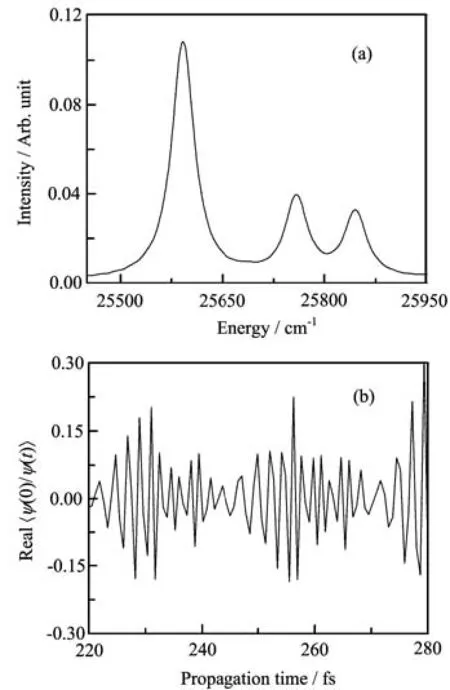
FIG.5(a)The solid line is the expanded portion of the calculated absorption spectra using the HamiltonianˆHRθsin Eq.(45)with FBST;the dotted line is from the model using the HamiltonianˆHRcsin Eq.(44)with FBSC;and the dashed line corresponds with the numerical results shown in Fig.1.(b)The real part of the auto-correlation function <ϕ(0)|ϕ(t)>.The solid and dotted lines are the results using the HamiltoniansˆHRθsandˆHRcswith FBST and FBSC,respectively.The dashed line corresponds with the numerical results shown in Fig.1.
Figure 7 illustrates the time-dependent norm calculated using the HamiltonianˆHRin Eq.(46)with the FBSC basis set.The exponential increase of the norm completely destroys the auto-correlation function and its Fourier transform,the absorption spectrum,loses its meaning.We do not show the resulting spectrum but note that the surviving peaks seem to stay at the right energy positions.
In this section,when the HamiltonianˆHRθsin Eq.(45)andˆHRθain Eq.(43)were used.The grid ranges were[1.8,3.9]in atomic units for R1and R2and[1.9, 3.1]in radians for θ.When the HamiltonianˆHRcsin Eq.(44)is used,the same grid ranges for R1and R2are used but[−0.9,0.25]for the variable C,i.e.,for cosθ. For each calculation,64×64×32 grid points are used(64 grid points along each radial coordinate and 32 along the angular coordinate).Convergence concerning grid ranges and grid spacing has been checked.
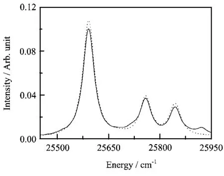
FIG.6 The solid line is the expanded portion of the calculated absorption spectra using HamiltonianˆHRθain Eq.(43) with FBST and the dotted line is the exact result shown in Fig.5.
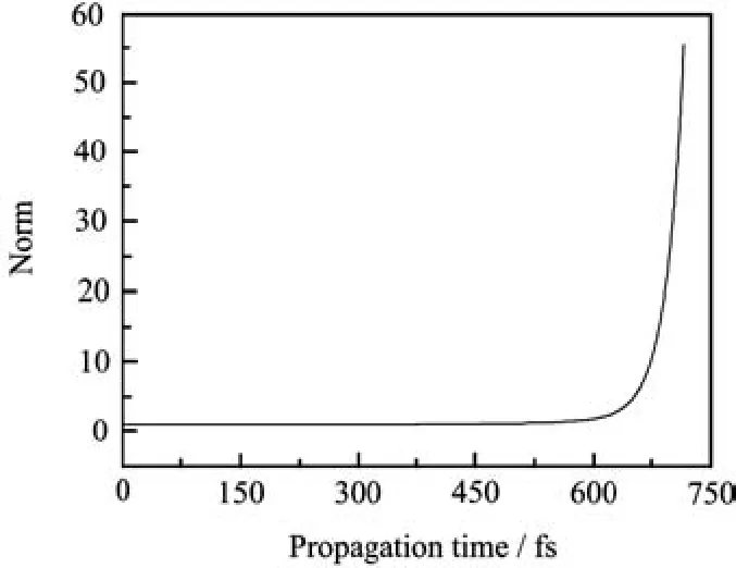
FIG.7 The time-dependent norm of the wavefunction obtained from evolving the non-hermitian matrix rsulting from the expanded HamiltonianˆHRin Eq.(46)with FBSC.
IV.DISCUSSION
We would like to note that the two absorption spectra shown in Fig.1 are not only virtually identical to each other,they are also virtually identical with those obtained using FFT and Hamiltonians expressed in Jacobi coordinates and in hyperspherical coordinates,where the convergence and the hermiticity of the Hamiltonian matrix has been carefully checked.Further,the lowest vibrational energies obtained using the relaxation method(imaginary time propagation method)[52]and the Hamiltonians in di ff erent coordinates,agree with each other better than 0.001 cm−1.This excellent agreement is in surprising contrast to the work of Katz et al.[28].This may demonstrate that the FFT is particularly suitable in the case where the PES is well bounded,for the PES of the A2A2state of the OClO molecule exhibits a deep well around the equilibrium geometry[24].
Among the numerical models,the calculation with the Hamiltonian in bond bond angle coordinates involves many more kinetic operators which greatly reduces the computation speed.Especially,numerical calculations using the transformed Hamiltonian in Radau coordinates in Eq.(45)are e ffi cient.It only requires three forward-backward FFTs for each Hamiltonian action,in contrast to the twelve needed for the symmetric HamiltonianˆHwsorˆHcsin bond bond angle coordinates!Further,the Hamiltonian in Eq.(45)does not mix local and non-local operator(s)of the same coordinate,which allows the application of the splitoperator method with the FFT technique to propagate the wavepacket.The numerical model using the HamiltonianˆHRθsin Eq.(45)with the FBST basis set not only gives a simple and e ffi cient way to numerical implementations but also signi fi cantly reduces the computation time[24,26].
We emphasize that both the analytic and numerical non-hermiticities of the Hamiltonian matrix discussed here give numerical implementations which are only conditionally stable.Especially in a long time propagation,the wavefunction norm violation may completely destroy the desired physical property of the simulated system.Interestingly,the non-hermiticity resulting from integration errors only always makes the norm of the propagated wavefunction increase exponentially,while the analytic non-hermiticity makes the norm oscillate.This may indicate that more complex and unphysical eigenvalues develop using an unsuitable Hamiltonian,which is re fl ected in the calculated spectra.We also note that,although the non-hermiticity of the Hamiltonian matrix makes the numerical model unstable and changes the heights of the physical peaks, the positions of the surviving physical peaks seem to be in the correct positions.In a Chebyshev propagation,the time-dependent norm of the wavefunction is useful for checking the convergence of numerical model. When a Hamiltonian and a suitable basis set have been correctly constructed,the norm of the time-dependent wavepacket should be well conserved.
V.SUMMARY
In this work,requirements on the forms of the Hamiltonians to be used with a discrete Fourier basis set is discussed.It is emphasized that for a chosen basis set,the Hamiltonian cannot be arbitrarily transformed.Otherwise,the resulting Hamiltonian matrix becomes nonhermitian,which may lead to numerical errors.Further, it is recommended to use symmetric forms of the operators in numerical calculations as here demonstrated for time-dependent wavepacket calculations using the FFT technique.Thus expanded forms of the Hamiltonian should also be avoided since they lead to nonhermitian Hamiltonian matrices due to integration errors.The in fl uence of these two kinds of non-hermiticity of the Hamiltonian matrix,i.e.,resulted from unsuitable Hamiltonian and purely resulted from integration errors,on 3D time-dependent wavepacket calculations were numerically investigated in bond bond angle and Radau coordinates.It was found that both of these non-hermiticities lead to the numerical calculation be-ing only conditionally stable.The non-hermiticity problem may be marginal in some cases,perhaps a short time propagation calculation.Although the conclusions drawn here,based on the OClO absorption spectrum calculations using Fourier basis sets,suggests that the numerical errors can be expected to be case-dependent, they should be generally applicable to calculations using DVR method.
VI.ACKNOWLEDGEMENTS
This work was supported by the National Basic Research Program of China(No.2013CB922200), the National Natural Science Foundation of China (No.21222308,No.21103187,and No.21133006),the Chinese Academy of Sciences,and the Key Research Program of the Chinese Academy of Sciences.
[1]R.Dawes and T.Jr.Carrington,J.Chem.Phys.122, 134101(2005).
[2]B.Poirier and L.C.Light,J.Chem.Phys.111,4869 (1999).
[3]B.Poirier and L.C.Light,J.Chem.Phys.113,211 (2000).
[4]B.Poirier and L.C.Light,J.Chem.Phys.114,6562 (2001).
[5]R.Meyer,J.Chem.Phys.52,2053(1970).
[6]D.Baye and P.H.Heenen,J.Phys.A 19,2041(1986).
[7]J.C.Light and Z.Ba˘ci´c,J.Chem.Phys.87,4008 (1987).
[8]H.Wei and T.Carrington Jr.,J.Chem.Phys.101,1343 (1994).
[9]J.C.Light and T.Jr.Carrington,Adv.Chem.Phys. 114,263(2000).
[10]D.Yu,S.L.Cong,D.H.Zhang,and Z.G.Sun,Chin. J.Chem.Phys.26,755(2013).
[11]G.Avila and T.Jr.Carrington,J.Chem.Phys.135, 064101(2011).
[12]X.S.Lin and Z.G.Sun,Chem.Phys.Lett.621,35 (2015).
[13]G.Nyman and H.G.Yu,Rep.Prog.Phys.63,1001 (2000).
[14]X.H.Liu,J.J.Lin,S.Harich,G.C.Schatz,and X.M. Yang,Science 289,1536(2000).
[15]H.S.Lee and J.C.Light,J.Chem.Phys.120,5859 (2004).
[16]J.Makarewicz,J.Phys.B 21,1803(1988).
[17]B.T.Sutcli ff e and J.Tennyson,Int.J.Quantum Chem. 91,183(1991).
[18]J.Z´u˜niga,A.Bastida,and A.Requena,J.Chem.Soc. Faraday Trans.93,1681(1997).
[19]H.G.Yu and J.T.Muckerman,J.Mol.Spectrosc.214, 11(2002).
[20]R.Schinke,Photodissociation Dynamics Spectroscopy and Fragmentation of Small Polyatomic Molecules, Cambridge University Press(1993).
[21]P.Marquetand,A.Materny,N.E.Henriksen,and V. Engel,J.Chem.Phys.120,5871(2004).
[22]N.E.Henrisken and V.Engel,Int.Rev.Phys.Chem. 20,93(2001).
[23]G.M.Krishnan and S.Mahapatra,J.Chem.Phys.118, 8715(2003).
[24]Z.Sun,N.Lou,and G.Nyman,J.Phys.Chem.A 108, 9226(2004).
[25]Z.Sun,N.Lou,and G.Nyman,J.Chem.Phys.122, 054316(2005).
[26]˘G.Barinovs,N.Markovi´c,and G.Nyman,J.Chem. Phys.111,6705(1999).
[27]Z.Sun,N.Lou,and G.Nyman,Chem.Phys.308,317 (2005).
[28]G.Katz,K.Yamashita,Y.Zeiri,and R.Koslo ff,J. Chem.Phys.116,4403(2002).
[29]R.Koslo ff,J.Phys.Chem.92,2087(1988).
[30]D.Koslo ffand R.Koslo ff,J.Comput.Phys.52,35 (1983).
[31]M.D.Feit,J.A.Jr.Fleck,and A.Steiger,J.Comput. Phys.47,412(1982).
[32]R.N.Dixon,Chem.Phys.Lett.190,430(1992).
[33]R.N.Dixon,J.Chem.Soc.Faraday Trans.88,2575 (1992).
[34]U.Manthe and H.K¨oppel,Chem.Phys.Lett.175,36 (1991).
[35]U.Manthe,H.K¨oppel,and L.S.Cederbaum,J.Chem. Phys.95,1708(1991).
[36]C.E.Dateo,V.Engel,R.Almeida,and H.Metiu, Comp.Phys.Comm.63,435(1991).
[37]C.E.Dateo and H.Metiu,J.Chem.Phys.95,7392 (1991).
[38]C.Woywod,Chem.Phys.Lett.281,168(1997).
[39]G.G.Balint-Kurti,R.N.Dixon,and C.C.Marston, Int.Rev.Phys.Chem.11,317(1992).
[40]R.C.Mowrey,Y.Sun,and D.J.Kouri,J.Chem.Phys. 91,6519(1989).
[41]D.Lemoine,J.Chem.Phys.101,10526(1994).
[42]˘G.Barinovs,N.Markovi´c,and G.Nyman,J.Phys. Chem.A 105,7441(2001).
[43]I.Tuvi and Y.B.Band,J.Chem.Phys.107,9079 (1997).
[44]B.Podolsky,Phys.Rev.32,812(1928).
[45]M.L.Boas,Mathematical Methods in the Physical Sciences,New York:Wiley,(1983).
[46]P.R.Bunker,Molecular Symmetry and Spectroscopy, Canada:NRC Research Press,(1998).
[47]R.D.Bardo and M.Wolfsberg,J.Chem.Phys.67,593 (1977).
[48]G.D.Carney,L.L.Sprandel,and C.W.Kern,Adv. Chem.Phys.37,305(1978).
[49]S.Carter and N.C.Handy,Mol.Phys.57,175(1986). [50]B.R.Johnson and W.P.Reinhardt,J.Chem.Phys. 85,4538(1986).
[51]K.A.Peterson,J.Chem.Phys.108,8864(1998).
[52]R.Koslo ff and H.Tal-Ezer,Chem.Phys.Lett.127,223 (1986).
猜你喜欢
杂志排行

CHINESE JOURNAL OF CHEMICAL PHYSICS的其它文章
- ARTICLE E ffi cient Separation of Ar and Kr from Environmental Samples for Trace Radioactive Noble Gas Detection†
- ARTICLE Spectrum Correction in Study of Solvation Dynamics by Fluorescence Non-collinear Optical Parametric Ampli fi cation Spectroscopy†
- I.INTRODUCTION
- ARTICLE High-Resolution Experimental Study on Photodissocaition of N2O†
- ARTICLE In situ Detection of Amide A Bands of Proteins in Water by Raman Ratio Spectrum†
- ARTICLE Photoelectron Spectroscopy and Density Functional Calculations of TiGen−(n=7−12)Clusters†