一种光滑粒子流体动力学数据的后处理方法

李付鹏，汪继文，欧 莽

（1.安徽大学计算智能与信号处理教育部重点实验室，安徽合肥 230039；2.安徽大学计算机科学与技术学院，安徽合肥 230039）

文章编号：1001⁃246X（2015）01⁃0033⁃07

一种光滑粒子流体动力学数据的后处理方法

李付鹏1，2，汪继文1，2，欧 莽2

（1.安徽大学计算智能与信号处理教育部重点实验室，安徽合肥 230039；
2.安徽大学计算机科学与技术学院，安徽合肥 230039）

提出一种光滑流体动力学数据后处理的三角网格化方法.首先确定流场中每个粒子作用域内的配对粒子集；再以当前粒子的配对粒子集为限定条件进行Delaunay三角剖分，可得到由粒子作为节点的三角形单元集；最后对“虚假”单元做过滤处理.算例表明复杂边界条件和严重变形的流体区域上的SPH计算结果都可用该方法处理.

光滑粒子方法；非凸区域；Delaunay三角化；后处理

0 引言

近年来，光滑粒子流体动力学（smoothed particle hydrodynamics，简称为SPH）方法［1］逐渐成为解决物理问题的一个有效工具，与传统的基于网格的数值方法，如有限差分、有限元、有限体积方法不同，这是一种典型的无网格拉格朗日数值方法，它利用核函数对物理问题进行近似处理，用离散的粒子来描述宏观连续分布微观仍为粒子的流体，而每个粒子则携带了其所在位置的流体的各种性质，如质量、密度、速度、能量等，算法节点可以任意分布，并非有某种网格联系在一起，这种自适应的特点使得该方法在模拟流体剧烈变形或间断问题时具有显著优势，目前方法的应用已扩展到气体动力学、不可压缩、爆炸、固体力学和弹性体等多个领域.然而，与该算法应用快速发展所不相适应的是，方法的数据后处理技术一直没有太大的发展，甚至可以说是一大难题［2］.如果将计算后的结果直接图形化，得到的是大量无组织的离散粒子，无法表现出流体的性态，更无法对流体的等值线（面）、流线图等分析，现有的比较成熟的基于网格的可视化技术也无法直接利用.目前，就我们查阅到的文献而言，有基于Splash、Paraview等软件开发的SPH后处理程序［3］，但这类软件较为专业，通用性不好，同时在流体力学方面的处理能力有限.

文献［4－5］提出了一种处理SPH数据后处理的方法，该方法先利用Delaunay三角剖分技术对离散数据三角化，然后根据每个单元中三个节点是否彼此为粒子作用对，决定是否将该单元从单元集中删除，从算例来看，这种方法是可行的.本文根据SPH算法的特点，对上述方法进行了改进，提出了一种更为简便的SPH数据后处理方法，以粒子支持域（影响域）为限定条件进行限定三角剖分（constrained Delaunay triangulation，简称为CDT或conforming Delaunay triangulation，简称为RDT），与文献［4－5］相比，方法减少了所生成的多余的三角形网格的数量，删除的空白的三角形网格也随之减少，提高了算法运算的效率.这样做另一个优点在于三角网格化输出的图形能够清晰地体现各粒子之间的影响关系，凡与某个节点（粒子）相关联的其它节点（粒子）均为数据输出时刻与该粒子有相互影响的粒子，而且方法更加简便易行，一般情况下不需要过滤“虚假”单元，简化了算法流程，增强了算法的适应性，验证结果表明方法稳定性好，凸区域和严重变形的非凸区域上的SPH计算结果都可用该方法处理.

首先介绍SPH方法中与数据三角化相关的几个概念以及数据后处理的特点；接下来阐述SPH数据三角化的算法思想和步骤；最后通过算例验证，得出结论.

1 SPH粒子支持域和粒子配对

SPH方法近似偏微分方程的过程包含两个步骤：核近似和粒子近似，核近似是通过对场函数及权函数积分实现，粒子近似是在一个有限区域内对所有粒子进行加权求和实现.对于场函数f（x），核近似和粒子近似可以分别表示为

其中变量x是位置矢量，变量h被称为光滑长度，W（x-x′，h）即为光滑核函数，变量h用来确定核函数的支持域，是核宽度的一种度量，核近似算子习惯用角括弧＜＞标记.场函数的导数可以采取与上述类似的方法求出，将场函数与其导数的粒子近似公式与实际应用的方程相结合，便可以求解特定的物理问题.

从以上公式可以看出，光滑核函数在SPH近似方法中起着重要作用，它决定了函数表达式的精度和计算效率.在核函数的表达式中有两个参数，分别为粒子的位置矢量和光滑长度，对于某个特定的粒子i而言，其周围粒子与该粒子的距离｜xi－x′｜＞κh时，W（xi－x′，h）＝0，式中κ是与点x处光滑函数相关的常数，此时场函数f（x）＝0，就是说，粒子i周围的粒子对粒子i没有影响；仅当" ｜x-x′｜≤κh时，W（xi－x′，h）≠0，粒子i周围的粒子对粒子i产生影响．SPH定义｜ x-x′｜≤κh所确定的以粒子i位置为中心的以κh为半径的区域为粒子i支持域．粒子i支持域内的所有点的信息都被用来决定粒子i的信息，支持域外的信息则对该点没有影响．支持域与粒子的光滑长度有关，光滑长度h与因子κ的乘积决定了该粒子的支持域．对于两个光滑长度相同的配对粒子i和j来说，粒子i和j彼此均在对方的支持域内.

给出了支持域的概念，可以很容易地确定粒子的配对粒子，对于给定的粒子，其支持域内的所有粒子均为该粒子的配对粒子.如果整个算法过程中光滑长度为常数，配对粒子互相影响，彼此互为配对粒子，而对于可变光滑长度的方法，配对粒子可能是单向的，即一个粒子是另一个粒子的配对粒子；反之未必成立，也就是说可能出现其中一个粒子对另一个粒子发生作用，但不是相互作用的，这违背牛顿第三运动定律，因此必须设法保证粒子间相互作用的对称性，否则会导致流场不守恒.

SPH支持域内粒子搜索算法常用的有全配对搜索法、链表搜索法、树形搜索法.

2 SPH数据后处理

对于基于网格的数值方法，生成网格的目的在于为数值计算提供一个高质量的网格，以便提高数值计算的精度，网格主要的目的是用于数值计算，尽管也包括数据结果的显示和数值分析；而无网格算法生成网格的目的仅仅在于数据结果的显示和数值分析.

两类数值方法的数据处理的目的不同，生成网格质量的要求也不相同.基于网格的数值方法要求三角剖分必须满足Delaunay优化准则，对于流场变量梯度变化较为剧烈的局部区域还需要进行加密处理，这样才能得到较好质量的计算网格；而SPH算法虽然同样要求三角剖分满足Delaunay优化准则，但还有一个更为重要的限定条件，就是三角化后的三角形单元的三条边应当是配对边，即构成该三角形的三个顶点（粒子）在互相的作用域之内，只有彼此相互作用或影响的粒子对相连（即构成三角形的一条边）才有意义，否则会导致流场的“非物质”区域被剖分的现象，两个粒子无互相作用，就表明它们之间没有物质接触，即没有质量.如果一个三角形单元中有一对节点（由粒子构成的三角形顶点）之间没有物质接触，就表明这个单元内部有间断，因此从连续介质力学的观点出发，该单元就是没有真实的流场，因此不是配对的粒子就没有必要生成三角形单元；因此SPH数据的三角剖分属于限定三角剖分.

常见的限定三角剖分有CDT和RDT两种类型.CDT是指剖分域的边界或内部限定边在三角剖分结果中出现并且不允许被细分，既不允许在剖分域中加入额外的点；RDT允许在域中加入点从而使得域的所有边界存在于剖分结果中.对SPH粒子点数据集可以用CDT或RDT方法三角化，但意义不同，SPH粒子点具有描述所求解的问题应具有的各物理量（质量、密度、压力等），因此如果数据集用于数值计算，就必须按照CDT的方法剖分，图形化的数据保持原有场域的各物理量不变；如果数据集用于视觉效果（比如游戏等），就可以按照RDT方法三角化，加入些许虚拟点，增强视觉效果.两个不同的方法必然产生不同质量的三角化的网格，CDT方法由于不允许加点，可能造成SPH数据集边界附近的三角形单元不满足Delaunay优化准则.RDT允许加入额外的点，SPH数据集域内的所有单元均符合Delaunay优化准则.

3 SPH粒子三角化算法

算法以SPH粒子支持域内的配对粒子为约束条件，以Delaunay三角剖分算法为基础生成二维三角化网格，剖分时Delaunay优化准则（最小角最大化或空外接圆特性）检查及其换边操作仅限定在配对粒子集合中.

设SPH数据输出时刻，SPH粒子的集合为P，三角化后的粒子集合为Q，算法具体描述如下：

1）首先根据粒子的支持域概念调用搜索算法检索粒子集合P，确定每个粒子的配对集合；

2）对配对后的粒子集合按照粒子的坐标排序，生成有序粒子点集；

3）从有序粒子点集中依序确定当前粒子，调用Delaunay算法对当前粒子及其配对集合中的粒子三角剖分，将参与三角剖分后的粒子依序加入到Q；

4）若当前粒子的配对集合中的元素（粒子）都已三角化，则从已经三角化的集合Q中依序确定新的当前粒子；

5）依次检测并删除当前粒子的配对粒子集合中与集合Q有交集的元素（粒子），对当前粒子配对集合中存留的元素（粒子）三角化处理，并将三角化后的元素（粒子）添加到Q集合中；

6）若当前粒子配对集合中的元素处理完毕，从Q集合中依序选取新的当前粒子，重复步骤5，直至遍历Q集合中的所有元素，算法结束.

需要说明的是：结束时，可能依然存在P中的部分元素（粒子）没有被三角化的现象，原因主要有以下两个方面：这部分粒子没有与其他的粒子相互作用，多表现为由于流体碰撞飞溅出去的粒子；另一种可能是这部分粒子与其它粒子没有物质接触，这部分粒子构成的流体与其它流体之间存在着间断或不连通的现象.此外，上述算法中最初参与三角剖分的粒子的选取很重要，如果最初参与剖分的是孤立粒子，由于孤立粒子周围没有配对粒子，将导致算法无法进行下去.这时要将该粒子直接删除，重新依序选择新的参与剖分的粒子.

另一点需要说明的是：后处理的精细化问题.由于对流体局部细节表现的需要或者视觉效果的需要，需要将粒子占据的区域离散的更细，从而使得物理量场的变化能被更精细地反映出来.表现细节可以采取粒子分裂技术［6］，基本的原则是在对粒子及新增粒子的物理量重新分配时，要遵循质量守恒和动量守恒；如果是为了视觉的需要（比如游戏等），可考虑加入些许虚拟点，增强视觉效果，上述两类处理都属于RDT类型的三角剖分，由于允许加入额外的点，SPH数据集域内的所有单元均符合Delaunay优化准则.后处理的精细化的方法［7］可以很容易地加入上述算法之中.

4 网格的质量

在基于网格技术的数值方法中，都非常重视剖分网格的质量，因为数值方法的计算精度都会不同程度的受到网格质量的影响，一般要求计算网格不能存在很小或很大的夹角.在二维网格中，就三角形剖分而言，一般用三角单位的外接圆半径与内切圆半径的比值或者用三角形单位的外接圆半径与最短边长的比值来度量网格单元的质量［8］，质量越好的网格剖分，三角形单元越接近于正三角形.

而在无网格方法中，网格化的目的不是用于数值计算，而是用于数据后处理，所以网格化的图形只要准确反应数值计算的结果就行了，对剖分的质量要求也与基于网格化的数值方法不一样，网格化后的图形一方面要能够表现出流场的运动的特征，另一方面又要能够体现出粒子之间的相互关系，这是最重要的两个目的.

5 算例

5.1 算例1

算法对文献［4］描述的算例进行了模拟.算例的计算域和初始粒子分布如图1所示，初始时刻所有粒子静止，没有外力作用，圆形液滴以某一初始速度匀速向下运动，图1－4显示了流场中的粒子在初始时刻、碰撞、融合、飞溅等时刻的分布和三角化后对应的各时刻的网格曲面图.没有对三角化后的网格作特殊处理，飞溅的粒子能够被算法有效的“过滤”，没有多余的单元，与文献［4］相比，不需要再对三角化后的网格再次“过滤”删除多余的单元.

图1 初始时刻粒子分布和网格曲面Fig.1 At t＝0.0s particle distributions and element sets derived by Delaunay triangulation

图2 2.5×10－3s时刻粒子分布和网格曲面Fig.2 At t＝2.5×10－3s particle distributions and element sets derived by Delaunay triangulation

图3 5.0×10－3s时刻粒子分布和网格曲面Fig.3 At t＝5.0×10－3s particle distributions and element sets derived by Delaunay triangulation

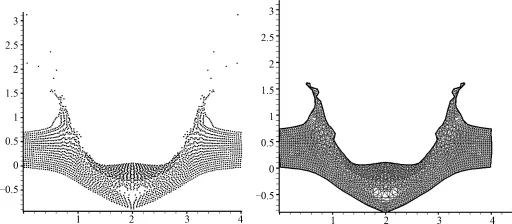
图4 12.5×10－3s时刻粒子分布和网格曲面Fig.4 At t＝12.5×10－3s particle distributions and element sets derived by Delaunay triangulation

5.2 算例2

二维圆溃坝问题.问题的求解区域是一个（0，50 m）×（0，50 m）的正方形，在正方形的中心是一个半径为11 m的圆柱面形坝体.初始时，坝内水深10 m，坝外水深1 m，且水是静止的.研究在坝体突然溃决（完全消失）后水的径向运动的规律.这一问题可以用来检验方法保持对称性的性能.SPH方法输出的数据进行网格化处理后再导入TECPLOT软件，得到时间为0.69 s时的水流自由表面图和水深等高线图，分别如图5和图6所示.从图5可知，本文所使用的SPH方法具有较好的对称性，也较好地显示了坝决后0.69 s时的水流形态，但对图6做进一步分析可知，在流场的局部区域，水深等高线与基于网格的方法［9－10］相比略显杂乱，这说明本文所使用的SPH方法还需要进一步改进.

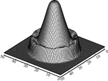
图5 水流自由表面Fig.5 Water surface profile after breaking of a circular dam

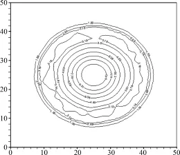
图6 水深等高线Fig.6 Contours ofwater height after breaking of a circular dam

5.3 算例3

二维部分溃坝问题.问题的求解区域是一个（0，200m）×（0，200m）的正方形，正中有一条大坝将水库和下游一分为二，上游水深10m，下游水深5m.大坝在距离水库一边95m处，突然有一段75m长的坝体溃决，要求模拟这部分坝体倒塌后水流的情况，该问题可以用来检验方法对于复杂边界的适应性.问题的平面图见图7.

SPH计算的粒子分布见图8.采用虚粒子来处理固定边界条件.把网格化后的数据导入TECPLOT软件，可得到坝体溃决后7.2s时的水流自由表面图和水深等高线图，如图9、10所示.从图可知，水流的整体形态和等高线的分布都与基于网格的数值方法［9，11］得出的结果基本保持一致，但在流体局部细节的表现上，本文所使用的SPH方法与传统的数值方法计算的结果还有一定的差异，如下游坝体溃决的两侧所形成的漩涡没有传统数值方法明显，边界附近的计算结果也需要进一步改善.这说明经过网格化方法处理后的数据，能够较为准确地表现出所使用的数值方法的性能，同时也能发现数值方法所存在的问题.

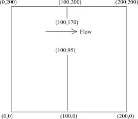
图7 二维部分溃坝问题Fig.7 Problem domain for partial dam break test

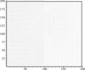
图8 二维部分溃坝问题的粒子分布Fig.8 Particle distributions in partial dam break test

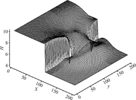
图9 水流自由表面Fig.9 Water surface profile after breaking of dam

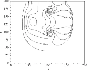
图10 水深等高线Fig.10 Contours ofwater elevation in partial dam break test

上述给出的算例表明，本文提出的SPH数据后处理的方法，在处理二维流体力学数值问题时具有一定的可行性，对于较为复杂的边界问题也能较好地处理.SPH数据通过网格化方法处理后，可以像基于网格的方法一样通过TECPLOT流体力学软件进行数值分析，数值分析的结果准确地反映了所使用的SPH算法的性能和存在的问题.

6 结论

提出一种光滑粒子流体动力学的二维数据后处理的方法，以粒子支持域为限定条件对离散粒子三角剖分，对于物质连通的流场区域，能够自动过滤飞溅的孤粒子，网格化后的数据一般不需要作特殊的处理，可以直接导入TECPLOT软件进行数值分析，算法简单易于实现.需要指出的是，本文不适合直接处理粒子飞溅较为严重的数值问题，这些飞溅的粒子可能会对流场的特性有较大影响，这类问题可采取粒子分裂方法，将粒子占据的区域离散成更多的粒子，尽可能地达到保留流场特性的目的.还需要指出的是，本文网格化后的数据表现的仅仅是流场的整体特征，无法表现SPH方法所特有的粒子飞溅、卷曲等细节特征.如何将网格化的方法与离散粒子相结合，图形化后的数据既能体现流场的整体特征，又能体现流场飞溅、卷曲等细节特征.这些是我们下一步的工作.

［1］ Randles PW，Libersky L D.Smoothed particle hydrodynamics：Some recent improvements and applications［J］.Computer Methods in Applied Mechanics and Engineering，1996，139（1）：375－408.

［2］ Massidda，Luca.ARMANDO，a SPH code for CERN⁃Some theory，a short tutorial，the code description and some examples ［R］.European Organization for Nuclear Research，CERN⁃AB⁃Note⁃2008⁃039⁃ATB，2008：1－36.

［3］ Biddiscombe J，Graham D，Maruzewski P，et al.Visualization and analysis of SPH data［J］.ERCOFTAC Bulletin，SPH Special Edition，2008，76：9－12.

［4］ Zheng Jun，Yu Kaiping，Wei Yingjie，Zhang Jiazhong.A general study on post⁃processing of smoothed particle hydrodynamics ［J］.Chinese Journal of Computational Physics，2011，28（2）：213－218.

［5］ 郑俊，于开平，张嘉钟，魏英杰.非凸区域上SPH计算结果后处理方法研究［J］.哈尔滨工业大学学报，2011，43（3）：12 －18.

［6］ Vacondio R，Rogers B D，Stansby P K.Accurate particle splitting for smoothed particle hydrodynamics in shallow water with shock capturing［J］.International Journal for Numerical Methods in Fluids，2012，69（8）：1377－1410.

［7］ Feldman J，Bonet J.Dynamic refinement and boundary contact forces in SPH with applications in fluid flow problems［J］. International Journal for Numerical Methods in Engineering，2007，72（3）：295－324.

［8］ 李海生.Delaunay三角剖分理论及可视化应用研究［M］.哈尔滨：哈尔滨工业大学出版社，2010：36－38.

［9］ Anastasiou K，Chan C T.Solution of the 2D shallow water equations using the finite volumemethod on unstructured triangularmeshes［J］.International Journal for Numerical Methods in Fluids，1997，24（11）：1225－1245.

［10］ Alcrudo F，Garcia⁃Navarro P.A high⁃resolution Godunov⁃type scheme in finite volumes for the 2D shallow⁃water equations［J］. International Journal for Numerical Methods in Fluids，1993，16（6）：489－505.

［11］ Wang Jiwen，Liu Ruxun.Finite volume methods for solving the problem of discontinuous solution［J］.Chinese Journal of Computational Physics，2001，18（2）：97－105.

Article ID：1001⁃246X（2015）01⁃0040⁃11

Abstract： A numerical model，which solves equations with spectral element method and resolves atmospheric near space，is developed.Model validations are performed.The spectral element model with atmospheric near space resolved（SEMANS）is integrated for 10 years under configuration of81 local elements in each projected face of cubed spherewith spectral approximation of8⁃th degree Gauss⁃Lobatto⁃Legendre interpolation polynomial and 66 vertical layers with top layer pressure 4.5×10－6hPa.Through verification against ERA⁃Interim reanalysis dataset from ECMWF（European Center for Medium⁃Range Weather Forecasts）and COSPAR（Committee on Space Research）international reference atmosphere 1986，it is found that SEMANS reproduces features of 2 wave⁃lengths pattern along zonal circle in the northern hemisphere and 1 wave⁃length pattern along zonal circle in the southern hemisphere at30 hPa；SEMANS reproduces zones of low temperature at about 100 hPa，0.001 hPa and high temperature at about 1 hPa，above0.000 1 hPa；SEMANSalso reproducesmain features of zonalmean zonalwind in January and July below 0.001 hPa level. Key words： spectral element；near space；atmospheric model；numerical simulation

0 Introduction

The atmosphere is divided into a number of layers associated with different features in temperature structure.The structure is determined primarily by the absorption of solar radiation［1］. Actions from military and commerce have extended greatly their scope in atmosphere in the vertical. Tomeet the demand for exploration and application，scientists proposed the concept of near space. Near space is the region of Earth′s atmosphere that lies between 20 and 100 km above sea level，encompassing the stratosphere，mesosphere，and the lower thermosphere.It is above where airliners fly in the sky but below orbiting satellites in the space.Satellites in the space cost high with long deployment cycles and are difficult to replenish after damage.Airliners in the sky can be attacked easily，have a low ability for survival and are also difficult to replenish after damage.Flight vehicles in the near space have high efficiency⁃cost ratio，goodmobility，little difficulty in payload technique and are easy for replenishment and maintenance.Since the distance from flight vehicles in the near space to earth surface is only about 1/20 to 1/10 of that from low orbit satellites to earth surface，sensors on those near space flight vehicles can detect low power transmissions that cannot be caught by satellites and it is easier to implementhigh resolution earth observation.Near space craft provides a rare air carrier for military applications such as airborne early warning，reconnaissance and monitoring.Itwill be an inevitable trend for early warning and tracking of cruisemissile to use near space craft.In addition，fighter air craft can fly up to 20 km；strategic ballistic missile flight canreach height of dozens of km；space airplanes can fly with a speed of12～25 Mach in an altitude of 30～100 km.These actions in near space demand meteorological supportwhich cannot be supplied by traditional numericalmodels and it becomes urgent and necessary to develop atmosphericmodels with the near space resolved.Under the context of global environment change，the atmospheric near space is subject to long⁃term changes due to bothman⁃made and solar variability effects.Man⁃made changes in the ozone layer and in the concentrations of other trace gases are expected to causemajor changes in the temperature structure within these regions，which will be most noticeable at high altitudes.These changes influence the atmospheric circulation，including possible effects on tropospheric climate，and may influence space operations and radio⁃wave communications［1］.Since much remains to be learned about this region，models that include many of the important effects related to dynamics，chemistry，and energetics，are important tools for carrying out related researches.

In community of geophysical computation，three numerical methods，finite difference method （FDM），spectral method（SM），and finite element method（FEM）are most frequently used. FDM，which is implemented through approximating differential quotientwith difference quotient，is efficient regard to programming and computational cost.The weakness of FDM is its low speed of convergence.SM，which ismore efficient than FDM［2］，is a high order，p⁃type weighted residual method.Since the basis functions of SM are global，it is usually applied to regular geometrical problem with smooth solutions.FEM，which is flexible for geometry and converges slowly as the number of the elements increased，is a low order，h⁃type weighted residual method.Spectral elementmethod（SEM），proposed by Patera，combine advantages of Galerkin spectralmethodswith those of finite elementmethods［3］.In SEM physical domain is broken up into several elements，which is usually triangular or quadrilateral［4－5］.Within each elementa spectral representation based on high order interpolation polynomials is used.Convergence is either obtained by increasing the degree of polynomials or by increasing the number of elements.A shallow water equation case showed that SEM provides not only good spational resolution and geometrical flexibity，but also affordability for long⁃range simulations［6］.SEM had been used for atmospheric dynamic core to perform three⁃dimensional climate modeling for low and middle atmosphere［7］.There have been many works on stratosphere simulation with numericalmodels discretized by FDM and SM.And it has been found that results from low⁃top models（model top below the stratopause）have very weak stratospheric variability on daily and interannual time scales，which leads to strongly underestimated frequency ofmajor sudden stratospheric warming events［8－9］.There are few atmosphericmodelswith model top above 100 km.Of which，the whole atmosphere community atmosphere model （WACCM）［10］and the whole atmospheremodel（WAM）［11］are themost popular ones.WACCM is an extension，upward through the thermosphere，of the national Center for Atmospheric Research （NCAR）community atmosphere model（CAM），which is an atmospheric component of the community earth system model（CESM）.WAM is also an extension，upward through the thermosphere，of the National Oceanic and Atmospheric Administration（NOAA）global forecast system（GFS）model as partof the integrated dynamics in the Earth's atmosphere（IDEA）project. TheWACCM and WAM are discretized with finite volumemethod（FVM）and SM，respectively.

In this work，we develop a spectral element model with atmospheric near space resolved （SEMANS）.A brief description of themodel is given in Section 1.Design of numerical experiment and datasets used for model validation are given in Section 2.Analysis on simulation results and model validation are shown in Section 3.In the last section，conclusions and discussions are given.

1 M odel discretization and physical processes

1.1 M odel equations

With static approximation，the control equations of SEAMNS are composed of a set of equations，which can be derived from their common forms appeared in text books of atmospheric dynamic.We have equation ofmomentum

equation of continuity

equation of temperature

and equation of constituent related towater（water vapor，cloud water，rain water，icewater and so on）

With appropriate choices for A and B，s is identical toσat the lowestmodel layer and p at high model layers.s is a hybrid ofσand p formiddlemodel layers.

The diagnostic equation for the geopotential is

whereφsurfis surface geopotential.

Tomake the equations complete，two diagnostic equations forandω

are added.Eqs.（1）－（8）make up themodel equations.

1.2 Spatial discretization

Themodel equations are discretized with SEM in the horizontal.To solve the polar problem inspherical coordinate，the earth sphere surface is projected onto its inner contact cubic and numerical computations are implemented in the projected local coordinates on elements of six faces.A 2⁃step projection（denoted by P）is needed to transform from spherical coordinate to projected local coordinates on elements（Step 1：From spherical coordinate to projected coordinates on six faces；Step 2：From projected coordinates on six faces to local coordinates on elements of six faces）.

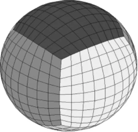
Fig.1 A cubed sphere（There are 81 elements on each projected face.）

The projected faces are divided into quadrilateral elements （Fig.1）.The quadrilateral element has been broadly used in such works of Taylor et al［12］，Giraldo et al［13］and Dennis et al［14］. Similar to that in Refs.［12－14］， Gauss⁃Lobatto⁃Legendre（GLL）gridding scheme is applied with SEMANS to facilitate the integration satisfying the Gaussian quadrature rule. Differences between these works lie in that，the configuration of the order of polynomial and the number of elements is different；themodel equations are different；the physics in thesemodels are different.Works of Refs.［12－14］deal with problems of single layer or multi⁃layers mainly within troposphere with simple physical process parameterization schemes adopted，whereas SEMANS can simulate the atmosphere up to the low thermosphere with complicated physical process parameterization schemes used.

The SEM is a kind of weighted residualmethod.Themodel equations are written in Galerkin form and then transformed to formula expressed in local coordinates on elements whose domain of definition is［－1：1；－1：1］.

The variables are interpolated as

Here，αaremodel variable such as u，v，T and qi，αijare expansion coefficients ofαand they vary with time，x and y are local coordinates on elements.The interpolation functions hiare Legendre cardinal functions.

In SEMANS，the spatial integrations are approximated by Gauss⁃Lobatto integration.Choosing Legendre cardinal functions as weight functions，the integration equations are discretized to equations of expansion coefficients of∂α/∂t．The solutions can be expressed with projection operator P as

where RHS means other items on the right hand side of equation.If we exchange the sequence of projection and temporal integration，the computation can be divided into 2 steps：

The first step is implemented within local elements and no data exchange between elements is needed.The computation in the second step needs data exchange between elements.

Themodel equations are discretized with FDM in the vertical.stop＝s1/2and sK＋1/2＝1．Thediscretization operator of∂/∂s isδs（X）k＝（Xk＋1/2－Xk－1/2）/（sk＋1/2－sk－1/2）and∂/∂s isδs（X）k＝（2πkΔsk）－1［（π）k＋1/2（Xk＋1－Xk）＋（π）k－1/2（Xk－Xk－1）］whereΔsk＝sk＋1/2－sk－1/2．

1.3 Physical processes

Zhang and McFarlane scheme［15］is used for deep convection.Park and Bretherton scheme［16］is used for shallow convection.A nonlocal diffusion scheme［17］is used for boundary layer parameterization.The near surface constant flux over land is calculated with Monin⁃Obukhov similarity theory and those over ocean water and sea ice are calculated with bulk formula.Below 60 km in altitude，solar radiation is computed withδ⁃Eddington approximation［18］and thermal radiation is computed with Ramanathan et al scheme［19］.Over 100 km，radiation heating rates from TIME⁃GCM（thermosphere ionospheremesosphere electrodynamics general circulationmodel）［20］are used. For height between 60 km and 100 km，weighted average of TIME⁃GCM results and radiation transfer output is used and weight coefficients are dependent onmodel layer.No chemical processes are considered at present.

1.4 Temporal integration scheme and boundary conditions

Leap⁃frog scheme is used for temperal integration.At boundaries of top and bottom，no flux conditions in which（π）1/2＝（π）K＋1/2＝0，are adopted.

2 Numerical experiments and datasets

Themodel atmosphere is divided into 66 layers with a pressure at the top 4.5×10－6hPa （Fig.2）.Each projected face is divided into 81 local elements and GLL interpolation polynomial of degree 8 is used to discretize the equation in each local element（Fig.3）.

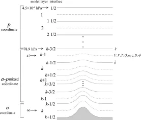
Fig.2 Vertical coordinate and model layers

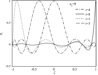
Fig.3 Gauss⁃Legendre⁃Lobatto interpolation polynomialswith degree 8

The data used for low boundary conditions andmodel initial values are all from the ERA⁃Interim dataset［21］.Dataset used for model validation are ERA⁃Interim dataset（from 1985 to 1994）and COSPAR（Committee on Space Research）International Reference Atmosphere1986（CIRA⁃86）［22］.

Initial values are from the atmospheric state at0 hour，0 minute，0 second of GMT（Greenwich Mean Time）on January 1st1989.Formodel layers above 1 hPa，values of variables such as zonal wind，meridional wind and temperature are identical to those of the highest model layer below 1hPa.Digital filter initialization［23］is used to reduce the initial imbalances and spurious gravity wave amplitude.The sea surface temperature，sea ice concentration，soil temperature and soilmoisture are all 12 monthly means of 1989，which are interpolated to model time needed within a year and used as bottom conditions.Land cover fraction and model terrain are interpolated from U.S. Geological Survey（USGS）dataset.

SEMANS has been integrated for 10 years and monthly mean model results are saved for analysis.During the integration，globalmean total energy（sum of sensible heat，potential energy，latent heat for phase change between cloud water and cloud ice，latent heat for phase change between vapor and cloud ice）and airmass（represented by surface air pressure）aremonitored every step.There is no obvious strange value found in theses variables.The globalmeanmonthly averaged surface air pressure is shown in Fig.4.It can be seen that the simulated seasonal variation of global mean airmass is reasonable and there is no obvious trend longer than a year.

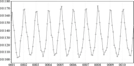
Fig.4 Globalmean monthly averaged surface air pressure（Unit of vertical axis is Pa and unit of horizontal axis is year.）

3 Simulation results

Since atmospheric data of observation is scarce above altitude of 10 hPa level，simulation results are verified for stratosphere below altitude of 10 hPa level only.SEMANS can reproduce the features of 2 wave⁃lengths pattern along zonal circle in the northern hemisphere and 1 wave⁃length pattern along zonal circle in the southern hemisphere（Fig.5）.The simulated strength of disturbance in the northern hemisphere is weaker than that of ERA⁃Interim and the simulated strength of disturbence in the southern hemisphere is similar to that of ERA⁃Interim.Compared to result from ERA⁃Interim，the simulated extent of lower value area near the equator enclosed by 23 800 gpm is smaller.

SEMANS reproduced main features of zonal mean zonal wind in January.The positions of westerly belt，easterly belt and large wind speed centers in January simulated by themodel coincide with those of ERA⁃Interim well.The simulated intensity ofwesterly jet in northern hemisphere below 100 hPa level and above 30 hPa level isweaker than those of ERA⁃Interim.The simulated intensity of easterly near the equator is also weaker than those of ERA⁃Interim（Figs.6（a），6（b））.

SEMANS also reproduced main features of zonalmean zonal wind in July.The positions of westerly belt，easterly beltand largewind speed centers in July simulated by themodel coincidewiththose of ERA⁃Interim well.The simulated intensity ofwesterly jet in southern hemisphere above 30 hPa level is stronger than that of ERA⁃Interim.The span of simulated easterly belt below 100 hPa near the equator is smaller than that of ERA⁃Interim（Figs.6（c），6（d））.

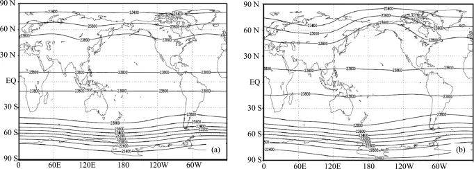
Fig.5 Distribution of geopotential height at30 hPa from（a）SEMANSand（b）ERA⁃Interim for 10⁃year average （Contour interval is 200 gpm.）

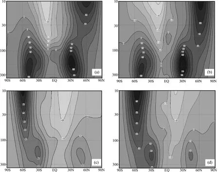
Fig.6 Distribution of zonalmean zonal wind from SEMANS（left）and ERA⁃Interim（right）in January（upper）and July （lower）for 10⁃year average（Contour intervals are 5 m·s－1for（a），（b）and 10 m·s－1for（c），（d）.）

The lower part（0～120 km）of CIRA⁃86，consisting of themonthlymean values of temperature and zonalwind with almost global coverage（80°N～80°S），is used for evaluation of SEMANS.As illustrated in Fig.7，SEMANS reproduces the zones of low temperature atabout100 hPa，0.001 hPa and high temperature atabout1 hPa；the characteristic ofhigh temperature above0.0001 hPa is alsoreproduced.But the simulated temperature at about 0.001 hPa is higher than that of CIRA⁃86 in January（Figs.7（b），7（a））.The high temperature center of 1 hPa level at North Pole is not reproduced by SEMANS in July（Figs.7（d），7（c））.

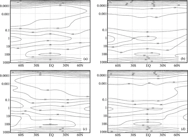
Fig.7 Distribution of zonalmean temperature from CIRA⁃86（left）and SEMANS（right）in January（upper）and July（lower）（Unit of vertical axis is hPa and contour interval is 20 K.）

Compared to CIRA⁃86，SEMANS reproduces the main features of distribution of zonal mean zonal wind below 0.001 hPa level，whereas there are much more discrepancies above that level （Figs.8（b），8（a）and 8（d），8（c））.These discrepancies are at least partly due to effect of exclusion of gravity wave in SEMANS.

4 Conclusion and discussion

A spectral elementmodel with atmospheric near space resolved was developed and preliminary work onmodel validation was done.Due to scarcity of observation data over10 hPa level，simulation results are verified against ERA⁃Interim reanalysis dataset for atmospheric stratosphere below 10 hPa level and reference atmosphere CIRA⁃86 for high levels.SEMANS reproduced the features of 2 wave⁃lengths pattern along zonal circle in the northern hemisphere and 1 wave⁃length pattern along zonal circle in the southern hemisphere at 30 hPa.SEMANS also reproduced themain features of zonalmean zonalwind in January and July.There areminute discrepancies between model results and ERA⁃Interim reanalysis dataset.Since there are differences even between reanalysis datasets from different sources，the discrepancies found here is thought to be acceptable.SEMANS reproduces the zones of low temperature at about100 hPa，0.001 hPa and high temperature at about 1 hPa and above 0.0001 hPa.But there is a spurious high temperature band around 0.2 hPa level.SEMANS reproduces the main features of distribution of zonalmean zonal wind below 0.001 hPa level，whereas there aremuch more discrepancies above that level.

Fig.8 Distribution of zonalmean zonalwind from CIRA⁃86（left）and SEMANS（right）in January（upper）and July（lower）（Unit of vertical axis is hPa and contour interval is 20 m·s－1.）

The chemical processes and gravity wave drag effects are not considered in SEMANSatpresent. To improve the performance of SEMANS，morework such as consideration of chemical processes and gravity wave drag effects and fine tuning ofmodel parameters needs to be done.

The advantage of SEM over FEM and FDM is in the exponential convergence.In practice，to improvemodel resolution，one can either keep the order of polynomial（denoted by N）fixed and increase the number of elements（denoted by K），or keep K fixed and increase N.In addition，one can reposition elements，keeping both N and K fixed，or change N in different elements.In simulation with spectralmodel，such cases as negative terrain height and negative specific humidity may occur due to discontinuity.This is ameliorated but can notbe avoided in SEM.In recent years，numerical model with FDM attracts many researchers'attention again due to advantages in implementation of parallelization and computation property（The amount of computation doesn't increase dramatically with enhancement of resolution）.

Acknowledgments：The work is sponsored by the Natural Science Foundation of China（Grant No.41276190）.The ERA⁃Interim reanalysis datasets are downloaded from the ECMWF data server website.We thank the two anonymous reviews for their suggestions.

［1］ Geller M A，Brasseur G P，Evans JV，etal.Upper⁃atmosphere and near⁃earth space research entering the twenty⁃first century［M］∥Board on Atmospheric Sciences and Climate Commission on Geosciences，Environment，and Resources，National Research Council.The atmospheric sciences entering the twenty⁃first century.Washington DC，USA：National Academy Press，1998：199－271.

［2］ Haidvogel D B，Robinson A R，Schulman E E.The accuracy，efficiency，and stability of three numerical models with application to open ocean problems［J］.JComp Phys，1980，34：1－53.

［3］ Patera A T.A spectral elementmethod for fluid dynamics：Laminar flow in a channel expansion［J］.J Comput Phys，1984，54：468－488.

［4］ Liu Xiying.Introduction of physical processes into a dynamic framework of spectral element and numerical experiment of medium range weather prediction［C］∥Zhou Liandi.Proceedings of the 20th National Seminar of Hydrodynamics，Beijing，China：Ocean Press，2007：224－230.

［5］ Liu Xiying.Numerical simulation of typhoon movement with a regional spectral element barotropic atmospheric model［J］.Chinese Journal of Computational Physics，2011，28：35－40.

［6］ Ma Hong.A spectral element basin model for the shallow water equations［J］.JComp Phys，1993，109：133－149.

［7］ Thomas S，Loft R.The NCAR spectral element climate dynamical core：Semi⁃implicit Eulerian formulation ［J］.Journal of Scientific Computing，2005，25：307－322.

［8］ Charlton⁃Perez A J，et al.On the lack of stratospheric dynamical variability in low⁃top versions of the CMIP5 models［J］.JGeophys Res Atmos，2013，118：2494－2505.

［9］ Austin J，Horowitz LW，Daniel Schwarzkopf M，etal.Stratospheric ozone and temperature simulated from the preindustrial era to the present day［J］.JClimate，2013，26：3528－3543.

［10］ Brakebusch M，Randall C E，Kinnison D E，et al.Evaluation of whole atmosphere community climate model simulations of ozone during Arctic winter 2004－2005［J］.JGeophys Res Atmos，2013，118：2673 －2688.

［11］ Wang H，Fuller⁃Rowell T J，Akmaev R A，et al.First simulations with a whole atmosphere data assimilation and forecast system：The January 2009 major sudden stratospheric warming［J］.JGeophys Res，2011，116：A12321.

［12］ Taylor M，Tribbia J，Iskandarani M.The spectral elementmethod for the shallow water equations on the sphere［J］.JComput Phys，1997，130：92－108.

［13］ Giraldo F X，Rosmond T E.A scalable spectral element Eulerian atmosphericmodel（SEE⁃AM）for NWP：Dynamical core tests［J］.Mon Wea Rev，2004，132：133－153.

［14］ Dennis J，et al.CAM⁃SE：A scalable spectral element dynamical core for the Community Atmosphere Model［J］.Int JHigh Perform Comput Appl，2012，26：74－89.

［15］ Zhang G J，McFarlane N A.Sensitivity of climate simulations to the parameterization of cumulus convection in the Canadian Climate Centre general circulation model［J］.Atmosphere⁃Ocean，1995，33：407－446. ［16］ Park S，Bretherton C S.The university ofwashington shallow convection and moist turbulence schemes and their impact on climate simulationswith the community atmospheremodel［J］.JClimate，2009，22：3449 －3469.

［17］ Holtslag A A M，Boville B A.Local versus nonlocal boundary⁃layer diffusion in a global climate model ［J］.JClimate，1993，6：1825－1842.

［18］ Briegleb B P.Delta⁃Eddington approximation for solar radiation in the NCAR Community Climate Model ［J］.JGeophys Res，1992，97：7603－7612.

［19］ Ramanathan V，Downey P.A nonisothermal emissivity and absorptivity formulation for water vapor［J］.J Geophys Res，1986，91：8649－8666.

［20］ Marsh D，Roble R.TIME⁃GCM simulations of lower⁃thermospheric nitric oxide seen by the halogen occultation experiment［J］.JAtmos Solar Terr Phys，2002，64：889－895.

［21］ Dee D P，Uppala SM，Simmons A J，etal.The ERA⁃Interim reanalysis：Configuration and performance of the data assimilation system［J］.Quart JR Meteorol Soc，2011，137：553－59.

［22］ Fleming E L，Chandra S，Shoeberl M R，et al.Monthly mean global climatology of temperature，wind，geopotential height and pressure for 0～120 km［R］.Technical Memorandum 100697，National Aeronautics and Space Administration，Washington D.C.，1988：1－56.

［23］ Chen M，Huang X Y.Digital filter initialization for MM5［J］.Mon Wea Rev，2006，134：1222－1236.

A Post⁃processing M ethod for Smoothed Particle Hydrodynam ics Data

LIFupeng1，2，WANG Jiwen1，2，OU Mang2
（1.Key Laboratory of Intelligent Computing＆Signal Processing，Anhui University，Hefei 230039，China；
2.Department ofComputer Science and Engineering，Anhui University，Hefei 230039，China）

A post processing method for smoothed particle hydrodynamics data is presented on basis of Delaunay triangulation. Pairing particle set in scope of each particle in flow field is confirmed，and then discretized by Delaunay triangulation on condition of present pairing particle set，which leads to a set of triangle elements with particles as nodes.At last non material units are filtered. Examples indicate that SPH resultwith complex boundary conditions and severe deformation of fluid region can be treated.

smoothed particlemethod；non convex region；Delaunay triangulation；post processing

A Spectral Element M odel w ith Atmospheric Near Space Resolved（SEMANS）

LIU Xiying，LIU Chunyan，YAO Shanshan

（College ofMeteorology and Oceanography，PLAUniversity ofScience and Technology，Nanjing 211101，China）

P435 Document code：A

O302

A

2014－01－24；

2014－06－18

安徽高校省级自然科学研究（KJ2013A009）资助项目

李付鹏（1974－），男，安徽阜阳，博士生，从事计算流体力学、计算机流体动画模拟研究，E⁃mail：lifupenganda＠163.com

Received date： 2014－01－24；Revised date： 2014－06－18

Received date：2013－10－21；Revised date：2014－08－29

Foundation item s：Supported by National Natural Science Foundation of China（41276190）

Biography：Liu Xiying（1970－），male，PhD，associate professor，major in atmospheric dynamics and numerical simulation，E⁃mail：liuxynj＠gmail.com