Bayesian Reliability Modeling and Assessment Solution for NC Machine Tools under Small-sample Data

YANG Zhaojun， KAN Yingnan， CHEN Fei，*， XU Binbin，CHEN Chuanhai， and YANG Chuangui

1 College of Mechanical Science and Engineering， Jilin University， Changchun 130025， China2 Key Laboratory of CNC Equipment Reliability Technique of Machinery Industry，Jilin University， Changchun 130025， China



Bayesian Reliability Modeling and Assessment Solution for NC Machine Tools under Small-sample Data

YANG Zhaojun1，2， KAN Yingnan1，2， CHEN Fei1，2，*， XU Binbin1，2，CHEN Chuanhai1，2， and YANG Chuangui1

1 College of Mechanical Science and Engineering， Jilin University， Changchun 130025， China
2 Key Laboratory of CNC Equipment Reliability Technique of Machinery Industry，Jilin University， Changchun 130025， China

Although Markov chain Monte Carlo（MCMC） algorithms are accurate， many factors may cause instability when they are utilized in reliability analysis； such instability makes these algorithms unsuitable for widespread engineering applications. Thus， a reliability modeling and assessment solution aimed at small-sample data of numerical control（NC） machine tools is proposed on the basis of Bayes theories. An expert-judgment process of fusing multi-source prior information is developed to obtain the Weibull parameters' prior distributions and reduce the subjective bias of usual expert-judgment methods. The grid approximation method is applied to two-parameter Weibull distribution to derive the formulas for the parameters' posterior distributions and solve the calculation difficulty of high-dimensional integration. The method is then applied to the real data of a type of NC machine tool to implement a reliability assessment and obtain the mean time between failures（MTBF）. The relative error of the proposed method is 5.8020×10-4compared with the MTBF obtained by the MCMC algorithm. This result indicates that the proposed method is as accurate as MCMC. The newly developed solution for reliability modeling and assessment of NC machine tools under small-sample data is easy， practical，and highly suitable for widespread application in the engineering field； in addition， the solution does not reduce accuracy.

NC machine tools， reliability， Bayes， mean time between failures（MTBF）， grid approximation，Markov chain Monte Carlo（MCMC）

1 Introduction*

1.1 Small-sample problem of NC machine tools

Numerical control（NC） machine tools are the foundation of the equipment manufacturing industry. Reliability has become the key common technology constraining the development of this industry. China has been the world's number one consumer and importer of NC machine tools for 10 consecutive years since 2002. China's machine tool industry， academic circle， and government believe that research on the reliability of NC machine tools is very important. Reliability technology includes reliability modeling and assessment， failure analysis， reliability design，and reliability allocation. In 2013， YANG et al［1］， conducted a comprehensive review of the development of research on the reliability of NC machine tools.

Reliability modeling and assessment is a prerequisite of other reliability techniques， and the data collected from a reliability test are the foundation of reliability modeling and assessment. For a long time， the field test has been the only means of reliability testing for the entire system of an NC machine tool［1］； this test usually requires considerable resources， especially time. The earliest work was implemented by KELLER， et al［2］， who collected field data on 35 computer numerical control machine tools over a period of three years. JIA， et al［3］， collected data on 24 machining centers for over a year， and YANG， et al［4］，collected field failure data on 12 machining centers for over five years from 2005 to 2010. Other cases can be found in Ref. ［1］.

Currently， field reliability tests on NC machine tools are mainly carried out by universities in association with manufacturing companies under the support of projects at the national level. Jilin University has accomplished and is implementing multiple tests. However， a new phenomenon has occurred in several of the tests. That is， the number of failures observed throughout a test or the corresponding data-sample size is extremely small that classic statistical methods are incapable of modeling and assessing reliability. Many reasons account for this new phenomenon， and the main one is that the reliability level of NC machine tools continues to improve as technologies develop. Thus，corresponding small-sample data are inevitable and arise frequently now and in the future. The problem of reliability modeling and assessment for NC machine tools under a small sample of data， the so-called small-sample problem，needs to be investigated and resolved immediately. Solving this problem is of great significance， especially for China.

Time between failures（TBF） is an important type of data，and mean TBF（MTBF） is the most important index representing the reliability level of NC machine tools. Since the time of KELLER， et al［2］， many other scholars，such as JIA， et al［3］， YANG， et al［5］， ZHANG， et al［6］， and CHEN， et al［7］， have adopted the two-parameter Weibull distribution to describe the TBF of machine tools. All of these scholars adopted classic statistical methods， such as least squares estimation（LSE） or maximum likelihood estimation（MLE）， to estimate the Weibull parameters（scale parameter α and shape parameter β）. The expectation of the Weibull distribution is usually adopted as the MTBF， which is calculated by the parameters' estimators.

When the data sample is large， using LSE or MLE can obtain accurate parameter estimators. However， when dealing with small samples， the estimators of LSE and MLE， especially for shape parameter β， are known to be significantly biased［8］.

1.2 Bayesian methods for the small-sample problem

Classic methods cannot be applied to the small-sample problem of NC machine tools. Although several scholars have proposed to adjust the estimators of classic methods through the use of adjustment factors［9-10］， these methods have not drawn much attention compared with Bayesian methods. Owing to the development in calculation techniques， especially the advent of Markov chain Monte Carlo（MCMC） algorithms， Bayesian methods have become the main tools to solve small-sample problems in the reliability field. In 2008， HAMADA， et al［11］， released a book that systematically presented the theories and applications of Bayesian methods in the reliability field.

Given the existence of many expensive， highly reliable，complex systems in aerospace and military equipment，small-sample data cases are common. Many Bayesian reliability modeling and assessment methods have been developed for these cases. For example， GUIKEMA and PATÉ-CORNELL［12］performed a Bayesian analysis of the future success frequency of the 33 major families of launch vehicles， including China's Long March family. GUIKEMA and PATÉ-CORNELL［13］also studied infancy problems for launch vehicles and pointed out that under a small number of launch attempts， the Bayesian approach exhibits an advantage over classic statistical approaches of yielding estimates. In another simulation-based research，GUIKEMA［14］proved that the predictive accuracy of Bayesian methods is better than that of classic methods for estimating the risk of failure for binary failure/no failure systems， such as strategic missiles. ANDERSON-COOK， et al［15］， presented a Bayesian approach that combines component， subsystem， and system data with expert judgment for reliability modeling and assessment of missile systems.

In contrast to aerospace products and military equipment that have well-developed reliability technology systems，NC machine tools still lack a complete reliability technology system［1］. Bayesian methods for the reliability of NC machine tools are scarce. PENG and HUANG， et al［16］， implemented an accelerated degradation test（ADT）on a machining center's milling head. The acceleration factor was derived， the two-parameter Weibull distribution was adopted to model the milling head's TBF， and a Bayesian reliability assessment method was developed to incorporate the information obtained in the ADT with available field data. However， given that the milling head is a comparatively simple component， the ADT plan and corresponding Bayesian method are unsuitable for the entire system of an NC machine tool consisting of many subsystems and components. Thus， the development of a Bayesian method of reliability modeling and assessment for the entire system of NC machine tools is necessary and of great significance.

After determining the problem， the reliability model， and model parameters， a Bayesian method of reliability modeling and assessment for NC machine tools will mainly involve three steps: （1） building the prior distributions of the Weibull parameters； （2） calculating the parameters' posterior distributions based on prior distributions， Bayes theorem， and the data； and （3） estimating the parameters based on the posterior distributions and calculating MTBF using the parameter estimators. These three steps are introduced in sections 1.3， 1.4， and 1.5， respectively.

1.3 Expert judgment and prior distributions

Compared with classic methods that rely only on present data， an obvious advantage of Bayesian methods is that they can incorporate prior information with present data. Prior information usually needs to be quantified into the parameters' prior distributions to take part in the calculation，and expert judgment plays an important role in building prior distributions. However， most published methods do not explain in detail how experts achieved the final prior distributions. For example， in Ref. ［11］， rocket scientists stated that the prior distribution of the success probability of the launch vehicle is uniform in the interval （0.1， 0.9）according to past data and their engineering expertise； no further description was provided. GUIKEMA， et al［12］，adopted uniform distribution in the （0， 1） interval as the prior distribution of the success probability of launch vehicles. PENG and HUANG， et al［16］， adopted uniform distribution in the interval （0， 10 000） as the prior distribution for the Weibull scale parameter when no direct prior information existed； however， they did not discuss why 0 and 10 000 were selected as the endpoints. MING， etal［17］， directly presented the estimated interval of a product's reliability based on expert panel and historical information without presenting the details.

Prior distributions have a significant influence on the accuracy of reliability assessment. Thus， one must systematically study how to obtain prior distributions to develop a complete and practical Bayesian method for NC machine tools. Eliciting expert judgment to form a prior distribution and reduce the subjective bias is an independent research area supported by abundant literature. For example， QUIGLEY， et al［18］， provided a comprehensive introduction of how to elicit prior distributions based on expert judgment. WALLS and QUIGLEY［19］developed an elicitation process for prior distributions of reliability growth models' parameters based on expert judgment. MEYER and BOOKER［20］at Los Alamos laboratory published a book on eliciting and analyzing expert judgment. Thus， applying the techniques in the area of eliciting expert judgment to NC machine tools would be innovative and would achieve the fusion of multi-source prior information and expert judgment；reliable prior distributions could be obtained.

Since neither of the Weibull parameters（α and β） has an obvious physical meaning and experts with sufficient practical experience in the machine tool industry may be unfamiliar with probability or reliability knowledge， asking experts to directly provide the parameters' prior distributions is unfeasible. An indirect approach is needed.

KAMINSKIY， et al［21］， pointed out that for the two-parameter Weibull distribution， prior information on α and β is particularly difficult to elicit， whereas prior information on the Weibull cumulative distribution function（CDF） is generally easier to obtain. Therefore， in Ref. ［21］，prior information was presented in the form of the intervals of CDF estimates at two fixed time points. The CDF estimates were then translated into the parameters' prior distributions through Monte Carlo simulation. However，considering that CDF values are values of probability，which remains too abstract for experts to understand， a comparatively larger subjective bias is inevitable if this method is applied to NC machine tools.

GARTHWAITE， et al［22］， advised that “experts should be asked questions about quantities that are meaningful to them and questions should generally concern observable quantities rather than unobservable parameters.” ALBERT，et al［23］， pointed out that “experts are much more comfortable with answering questions based on time， which corresponds to observable quantities.” KADANE， et al［24］and LOW-CHOY， et al［25］， also advised the use of indirect means， that is， to elicit expert judgment on observable quantities and then infer the parameters based on the judgment.

The preceding discussion indicates that in Weibull CDF，time is a quantity that has a physical meaning； it is more perceivable and observable for experts than probability. Thus， we propose a new method wherein experts make a judgment on time， and then this judgment is translated into the Weibull parameters' prior distributions.

1.4 Calculating the posterior distributions of parameters

The combination of prior distributions and the data is implemented by the Bayes theorem， and the objective is to calculate the parameters' posterior distributions. Considering that the Weibull probability distribution function（PDF） has a complex form and the two Weibull parameters are both treated as random variables，“high-dimensional” integration having no closed form will occur in the calculation process. The corresponding formulas are illustrated in detail in section 3.

“Conjugate distribution” is an analytic method of simplifying “high-dimensional integration.” However， the fundamental result obtained by SOLAND［26］indicates that the Weibull distribution does not have a conjugate continuous joint prior distribution. No analytic solutions are available for the posterior distributions， but parameter estimations are based on posterior distributions. Further parameter estimators cannot be obtained analytically if posterior distributions do not have analytic solutions. First，a numerical method is required to solve the posterior distributions. Second， parameter estimation is implemented based on the numerically solved posterior distributions. MCMC algorithms（simulation） and the grid approximation method are two suitable choices.

MCMC algorithms are a general class of computational methods utilized to generate values from posterior distributions to form a Markov chain［11］. Common MCMC algorithms include Metropolis algorithms［27］， Metropolis-Hastings algorithms［28］， Gibbs samplers［29］， and Slice sampling［30］. However， when facing a specific problem in reality， researchers need to develop a specific algorithm based on the principles of common MCMC algorithms. Sometimes， a hybrid algorithm incorporated with different algorithms is needed. For example， GUPTA， et al［31］，developed a hybrid algorithm combining the Metropolis algorithm and the Gibbs sampler to simulate the posterior distributions of the Weibull extension model's parameters. SOLIMAN， et al［32］， developed a Metropolis-Gibbs hybrid algorithm to simulate the posterior distributions of the parameters of the modified Weibull distribution.

Many factors should be considered in successfully developing and implementing an MCMC algorithm. These factors include determining the burn-in period， selecting appropriate proposal distributions or initial values， and monitoring the convergence of a Markov chain［11］. Developing a specific MCMC program for a specific problem is thus difficult. Several software packages have emerged to help researchers； an example is the free software package WinBUGS. In WinBUGS， the Bayes problem needs to be modeled in a language called BUGS language. A BUGS model is then created， and the expert system on WinBUGS selects a suitable MCMC algorithmaccording to the BUGS model［33］. For complex problems，the usual algorithm WinBUGS selects is slice sampling proposed by NEAL［30］in 2003. However， as indicated in the user manual of WinBUGS， MCMC may fail. That is，any of the factors mentioned above could make the MCMC algorithm unstable or even crash. Thus， an MCMC algorithm， whether it is developed manually or by WinBUGS， usually requires the user to have a sufficient mathematical background and excellent programming ability. This condition prevents Bayes methods from being applied extensively in the reliability engineering field of NC machine tools.

By contrast， the grid approximation method can express the posterior distribution in a direct， explicit， approximate form. According to the introduction by KRUSCHKE［34］， the basic principle of grid approximation is to discretize the continuous variables. High-dimensional integration can be simplified as a summation， and further parameter estimation can be calculated directly. Compared with MCMC， grid approximation is easy to understand and practical to apply. Nevertheless， no study has discussed the application of grid approximation to the two-parameter Weibull distribution. To provide engineers who lack a statistical background with a suitable tool， the grid approximation method is applied to the two-parameter Weibull distribution in this study； the posterior distributions are solved， and the corresponding formulas are derived.

1.5 Estimations of parameters and MTBF

Parameter estimations are comparatively easy given the posterior distributions. Generally， the expectation of a parameter's posterior distribution is regarded as the Bayes point estimator of this parameter. In section 5， the formulas to calculate the point estimators and 90% credible intervals are derived based on posterior distributions obtained through grid approximation.

Section 6 shows the application of the proposed method developed in sections 2， 3， 4， and 5 to a real， small data sample. The same case is also modeled in WinBUGS in BUGS language； the BUGS code is developed， and the corresponding MCMC simulation is run with the same data sample for comparison.

2 Building the Weibull Parameters' Prior Distributions

2.1 Weibull distribution and its functions

The CDF of the two-parameter Weibull distribution，P=F（t）， is provided by Eq. （1）:

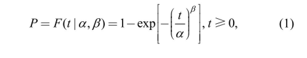
where α＞0 is the scale parameter， β＞0 the shape parameter，and θ = （α，β） is the parameter vector.

According to the discussion in section 1.3， the inverse function of CDF， t=F-1（P）， is provided by Eq. （2）:

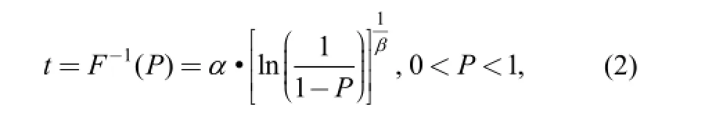
where t （time or possible observations of TBF） is the output and the value of CDF， P， is the input or exposure. Based on Eq. （2）， a process of eliciting expert judgment and presenting prior information in the form of intervals of time at fixed exposures is developed in section 2.2.

2.2 Elicitation of expert judgment

A structured， complete elicitation process of expert judgment includes many definitions and details， which can be found in Refs. ［18-20］. However， this paper presents two innovative definitions explained as follows.

“Target System” refers to the NC machine tool to be studied. “Reference System” refers to an NC machine tool that has sufficient historical data and is similar to the Target System in the following aspects: reliability， type， model，structure， and functions. An ideal situation is that the Target System is a modified model of the Reference System.

We let P=F0（t） and t=F0-1（P） denote the Target System's CDF and its inverse function； we let P=F1（t） and t=F1-1（P）denote the Reference System's CDF and its inverse function. The Weibull parameters for the Reference System are available based on historical data. Similar to the method in Ref. ［22］， two fixed exposures （P1and P2） are specified for the Reference System. According to O'HAGAN， et al［35］，the two most frequently assessed quantities are the 25th and 75th percentiles. Therefore， we adopt P1=0.25 and P2=0.75. Based on Eq. （2）， two time values， t11=F1-1（P1）and t12=F1-1（P2）， can be obtained（see Fig. 1）.

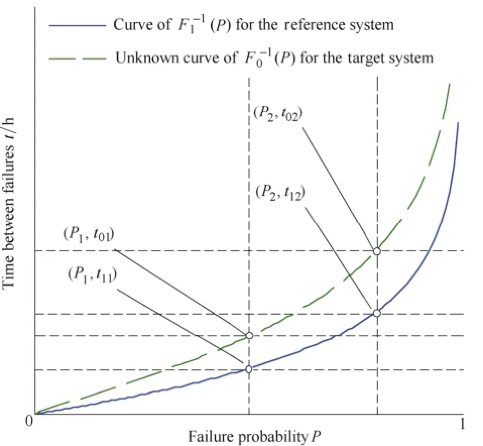
Fig. 1. Curves of Eq. （2） for the target and reference systems

A formal interpretation for points （P1， t11） and （P2， t12） in Fig. 1 is as follows: the probability that the TBF of theReference System is less than t11is P1， and the probability that the TBF of the Reference System is less than t12is P2.

An informal but intuitive interpretation for （P1， t11） and（P2， t12） is as follows: suppose that there are 100 similar Reference Systems being tested under the same situation；any single Reference System will be removed from the test for good after its first failure. A total of 100×P1Reference Systems are removed when t11（h） have elapsed. A total of 100×P2Reference Systems are removed when t12（h） have elapsed.

Each expert has a unique knowledge background. For example， an expert may be very familiar with reliability and statistical theories， whereas another one may be a machine operator with sufficient practical experience. Thus，considering the differences in knowledge background， this paper presents a formal set of questions （Q1， Q2） and an informal set of questions （Q1*， Q2*）， where Q1 is equivalent to Q1*and Q2 is equivalent to Q2*. Each expert may opt to answer any one set according to his own preference.

（1） First set of questions（see Fig. 1）

Q1: For the function t=F0-1（P） of the Target System， the estimate of time at fixed exposure P1is denoted as t01. What are the minimum（Lt01） and maximum（Ut01） values of t01？

Q2: For the function t=F0-1（P） of the Target System， the estimate of time at fixed exposure P2is denoted as t02. What are the minimum（Lt02） and maximum（Ut02） values of t02？

（2） Second set of questions（see Fig. 1）:

Suppose that there are 100 similar Target Systems being tested under the same situation； any single Target System will be removed from the test for good after its first failure.

Q1*: How long does it take until the number of removed Target Systems reaches 100×P1？ Provide the minimum and maximum values of this duration.

Q2*: How long does it take until the number of removed Target Systems reaches 100×P2？ Provide the minimum and maximum values of this duration.

Fig. 1 presents the curves ofbased on Eq. （2）. The figure provides experts an intuitive reference.

The elicitation process of expert judgment mainly consists of three stages.

The first stage is collecting multi-source prior information. Multi-source prior information generally belongs to 8 categories: （1） basic information（information on type， model， structure， manufacturer， and users）； （2）degree of multifunction of a product（more functions affect reliability）； （3） manufacturer's technology level（capabilities of designing and manufacturing）； （4） complexity of the product's structure； （5） degree of maturity of the product；（6） cost of the product （cost of the entire system and subsystems）； （7） user's degree of satisfaction of the product；and （8） operational performance of the product（feedback of operation and maintenance personnel）.

The second stage involves asking experts to receive and process the multi-source prior information.

The final stage is providing estimated， quantified answers. The three stages of the process are illustrated in Fig. 2.

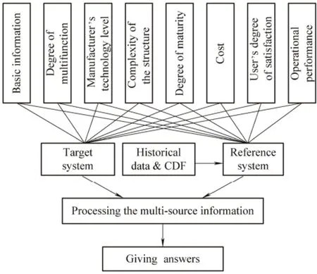
Fig. 2. Illustration of the elicitation process of expert judgment

2.3 Combination of expert judgments

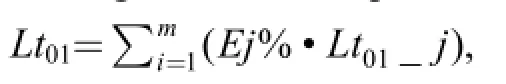
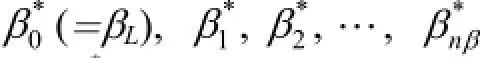
2.4 Building prior distributions

For the Target System， the final answer of expert judgment is believed to be equivalent to the judgment on the Weibull parameters. That is， the expert panel has already implicitly provided the intervals ［αL， αU］ and ［βL，βU］ in which α and β lie. Intervals ［αL， αU］ and ［βL， βU］ are provided by providing ［Lt01， Ut01］ and ［Lt02， Ut02］. Thus，mathematical skill is needed to transform ［Lt01， Ut01］ and［Lt02， Ut02］ into ［αL， αU］ and ［βL， βU］.

First， given the specified P1and P2， any pair （t01， t02）consisting of values obtained from ［Lt01， Ut01］ and ［Lt02，Ut02］， respectively， will determine a pair （α， β）. The derivation is as follows.

Substituting （P1， t01） and （P2， t02） into Eq. （1） respectively yields Eqs. （3） and （4）:

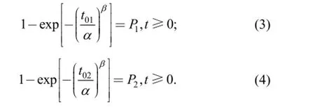
Thus， β and α can be obtained:

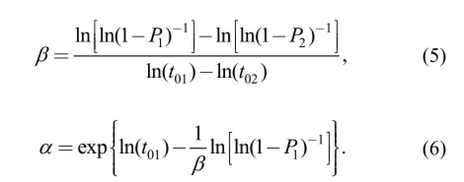
The transformation from pair （t01， t02） to pair （α，β） is achieved with Eqs. （5） and （6）. Based on point-to-point transformation， the transformation process from interval to interval， which is a Monte Carlo algorithm， is proposed.

（a） A value of t01in ［Lt01， Ut01］ and a value of t02in ［Lt02，Ut02］ are randomly selected.

（b） The values of （α，β）， which are denoted as （α1， β1），are calculated according to Eqs. （5） and （6）.

（c） Steps （a） and （b） are repeated N-1 times， and the values of （αi， βi） are recorded each time， where i=2， 3…N（e.g.， N=1000）.

（d） The minimum and maximum values of ｛αi｝ and ｛βi｝are determined.

（e） ［αL， αU］ = ［min（αi）， max（αi）］ and ［βL， βU］ = ［min（βi），max（βi）］.

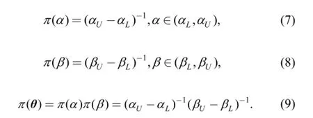
For NC machine tools， α and β have their own range of value. However， no certainty exists as to which value could be the true value because of the lack of knowledge and information. The relations of the two parameters are also uncertain. Therefore， in accordance with BERGER［36］， we assume that α， β are uniformly and independently distributed. For the Target System， the prior distributions（PDF） of the Weibull parameters and parameter vector are presented as follows:

3 Posterior Distribution and Highdimensional Integration

The theoretical formulas for the Weibull parameter vector's posterior distribution can be derived via the Bayes theorem in combination with the data. In this study， each data point is complete without censoring. The case where censored data exist will be studied in the future.

The PDF of the two-parameter Weibull distribution is provided by Eq. （10）:

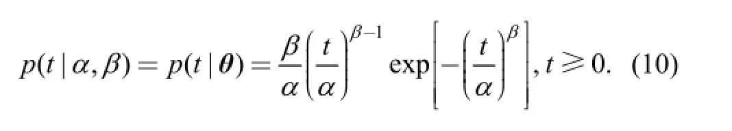
π（θ） denotes the prior distribution of parameter θ， and the random variable T denotes the complete TBF. An observation of T is denoted as tr， r=1， 2，…， n. Thus， the data sample is denoted as t=（t1， t2，…， tn）. The posterior distribution of θ is denoted as π（θ | t）.

Substituting data point trinto Eq. （10） reveals its contribution to the likelihood function:

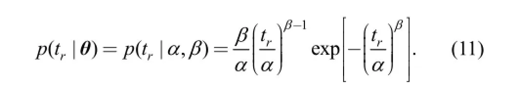
Likelihood function p（t | θ） is expressed by Eq. （12）:

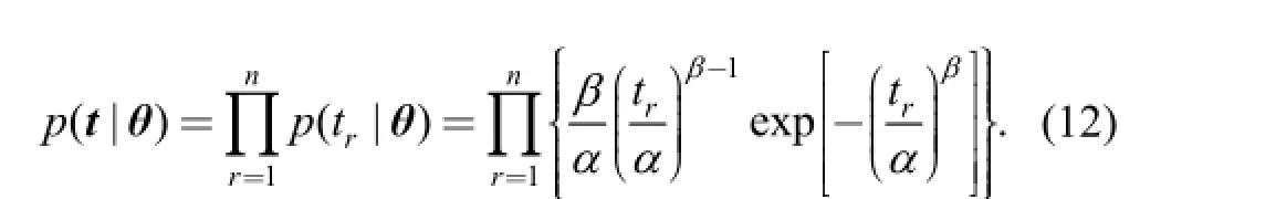
The marginal distribution of t is provided by Eq. （13）:

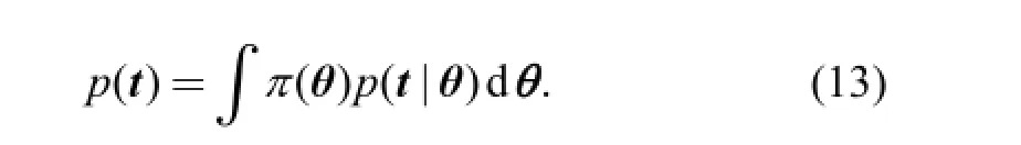
Based on the prior distribution， likelihood function， and marginal distribution of data， the parameter's posterior distribution， （|），πθ t can be obtained via Bayes theorem，which is shown in Eq. （14）:

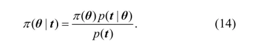
When θ=（α， β）， substituting Eqs. （12） and （13） into Eq.（14） yields the theoretical formula for the Weibull parameter's posterior distribution:

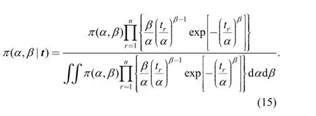
However， Eq. （15） does not have an analytic solution for the following reasons: （1） the denominator of the right-hand expression involves a double integral， （2） both α and β are random variables， and （3） the integrated function has a complex form. Thus， the integral is the so-called“high-dimensional integration，” which cannot have a closed form.

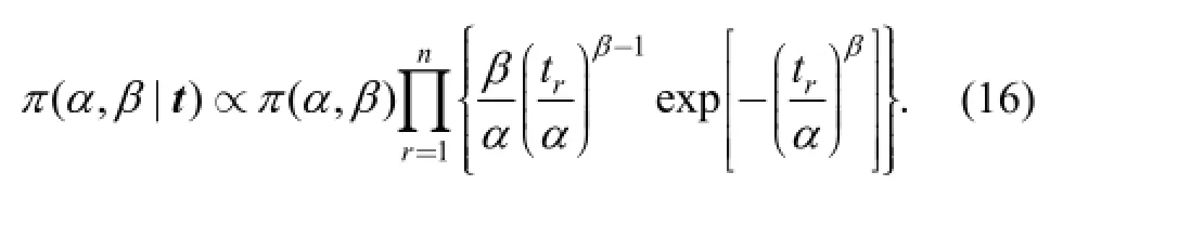
Given that the denominator of the right-hand expression of Eq. （15） is a constant， Eq. （15） can be written as Eq. （16），which is a basis of developing an MCMC algorithm:

4 Posterior Distributions Based on Grid Approximation

In this section， the principle of grid approximation is applied to the two-parameter Weibull distribution.

4.1 Approximating the prior distributions

The probability mass functions， πm（αi） and πm（βj）， are defined by Eqs. （17） and （18）:

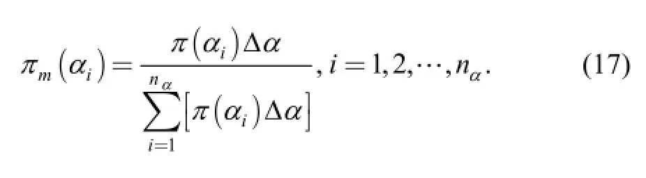
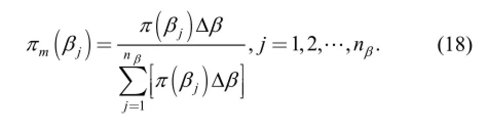
The domains of πm（αi） and πm（βj） are ｛αi｝ and ｛βj｝. Obviously， ∑πm（αi）=1 and ∑πm（βj）=1. Therefore，probability mass functions πm（αi） and πm（βj） are adopted as the approximate prior distributions of α and β， respectively.

We let θi，j=（αi， βj）. Probability mass function πm（θi，j） is defined by Eq. （19）:

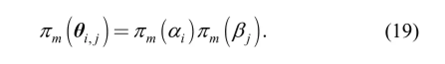
The domain of πm（θi，j） is denoted as ｛θi，j｝=｛（αi， βj）｝， i=1，2，…， nα， j=1， 2，…， nβ. Apparently， ∑∑πm（θi，j）=∑∑［πm（αi）πm（βj）］=1. Therefore， probability mass function πm（θi，j） is adopted as the approximate prior distribution of θ.

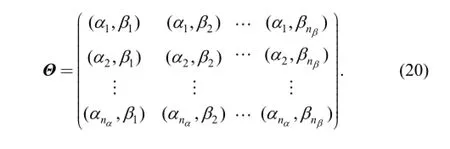
For deeper understanding， the domain of πm（θi，j） is denoted by matrix Θ. The total number of elements is nΘ=nα×nβ:

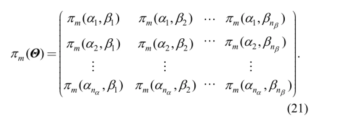
The probability mass at each point θi，j=（αi， βj） is also displayed in matrix πm（Θ） called “the prior distribution matrix.”:

4.2 Calculating the posterior distribution of θi，j

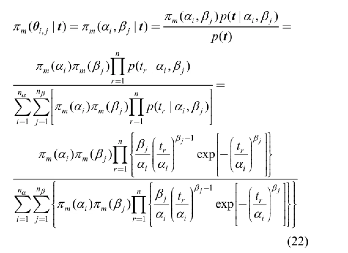
Given the data sample t=（t1， t2，…， tn）， the posterior distribution of θi，j=（αi， βj） can be obtained via the Bayes theorem. Given that θi，jis discrete， the Bayes theorem in Eq.（15） is rewritten into a discrete form by Eq. （22）:

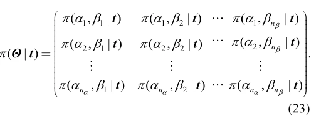
According to Eq. （22）， the posterior probability mass can be calculated and denoted as πm（θi，j|t） or πm（αi， βj|t） at each θi，j=（αi， βj）. The results are displayed by a matrix called the“posterior distribution matrix.”

4.3 Posterior marginal distributions of αiand βj

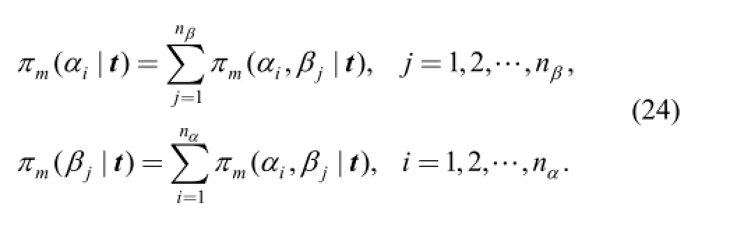
Based on the posterior distribution matrix in Eq. （23）， the posterior marginal distribution for a certain αior βjcan be denoted as πm（αi| t） or πm（βj| t） and calculated by Eq. （24）:

5 Estimation Based on Posterior Distributions

5.1 Point estimators of the Weibull parameters

Generally， Bayesian point estimation is related to a loss function indicating the loss coming up when the estimator deviates from the true value［37］. Loss functions are of many types. When parameter α （for example） is one-dimensional，the loss function can often be expressed as Eq. （25）:

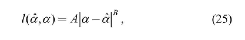
where A＞0 and B＞0. If B=2， the loss function is quadratic and is called a squared-error loss function（shown as Eq.（26））:

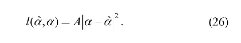
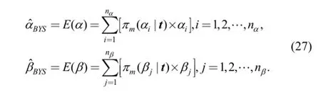
Refs. ［37， 38］ have proven that in a one-dimensional case and for a squared-error loss function， the Bayes estimator is simply the posterior mean， which can minimize the posterior risk. Thus， squared-error loss functions are adopted in the current study for α and β. Considering that both are one-dimensional， the posterior means of α and β are regarded as the point Bayesian estimators and provided by Eq. （27）:

5.2 Estimating the parameters' credible intervals

Compared with classic methods， a significant advantage of the Bayesian method is that the credible （confidence）intervals are easy to obtain. Given that ｛αi｝=｛α1， α2，…，αnα｝， i=1， 2，…， nα； ｛βj｝=｛β1， β2，…， βnβ｝， and j=1， 2，…，nβ. The posterior probability mass of each αior βjis obtained by Eq. （24）. Thus， when 90% is specified as the credible level， two equations can be presented:

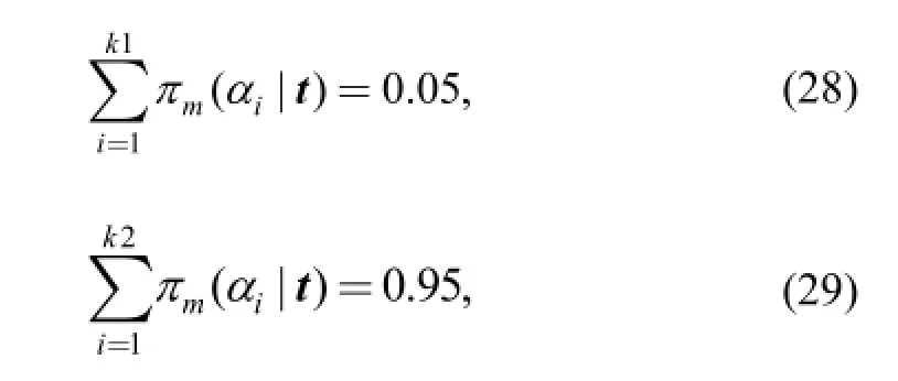
where k1 and k2 are two positive integers to be calculated. The interval ［αk1， αk2］ is the 90% credible interval of α.

Similarly， for β， two equations can be presented:

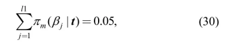
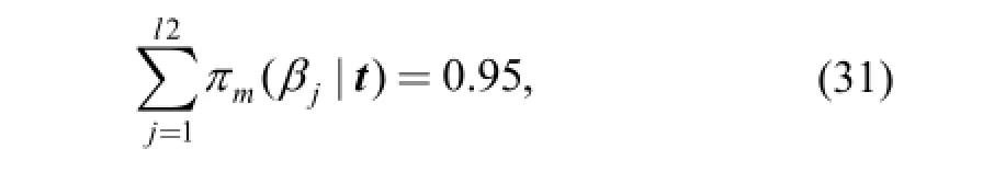
where l1 and l2 are two positive integers to be calculated. The interval ［βl1， βl2］ is the 90% credible interval of β.

6 Actual Application and Comparison

6.1 Target system

From October 26， 2013， to April 30， 2014， a field reliability test was conducted on a single NC machine tool，the type of which is NC turret punch. For confidentiality， its model is denoted as “Target.” Only four complete TBFs were observed. The data are shown in Table 1.

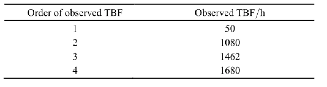
Table 1. Small-sample data of the Target System

6.2 Expert panel

The expert panel consists of an assessor responsible for leading the entire elicitation process， a data collector responsible for observing the failures and recording the data， a managerial expert to help the assessor arrange affairs and meetings， and three technical experts identified by the assessor in association with the managerial expert. The definitions of the above roles are obtained from Refs.［19-20］.

ce system

The expert panel identified a model of NC machine tools as the Reference System； the type is also NC turret punch，and its model is denoted as “Reference” for confidentiality. The Target is a modified model of the Reference.

Historical data on the Reference were obtained from a field reliability test on 10 copies. The test was implemented from February 18， 2012， to November 18， 2014. Eighteen complete TBFs were observed.

6.4 Raising specific questions

The TBF of the Reference was modeled by the two-parameter Weibull distribution based on the historical data in Table 2 and LSE. The details of LSE on Weibull distribution can be found in Ref. ［39］. The parameter estimators are α=426.086 4 and β=1.656 6.

First， two fixed values of exposure were specified as follows: P1=0.25 and P2=0.75. For the Reference，t11=200.850 3 h and t12=518.953 2 h as calculated with Eq.（2）.

For the two points（P1， t11）=（0.25， 200.850 3） and（P2， t12）=（0.75， 518.953 2）， the formal interpretation is as follows: the probability that the TBF of the Reference is less than 200.850 3 h is 0.25， and the probability that theTBF of the Reference is less than 518.953 2 h is 0.75. The informal interpretation is as follows: Suppose that there are 100 similar References being tested under the same situation， and any single Reference will be removed from the test for good after its first failure. Then， a total of 25 References are removed when 200.850 3 h have elapsed； 75 References are removed in total when 518.953 2 h have elapsed.

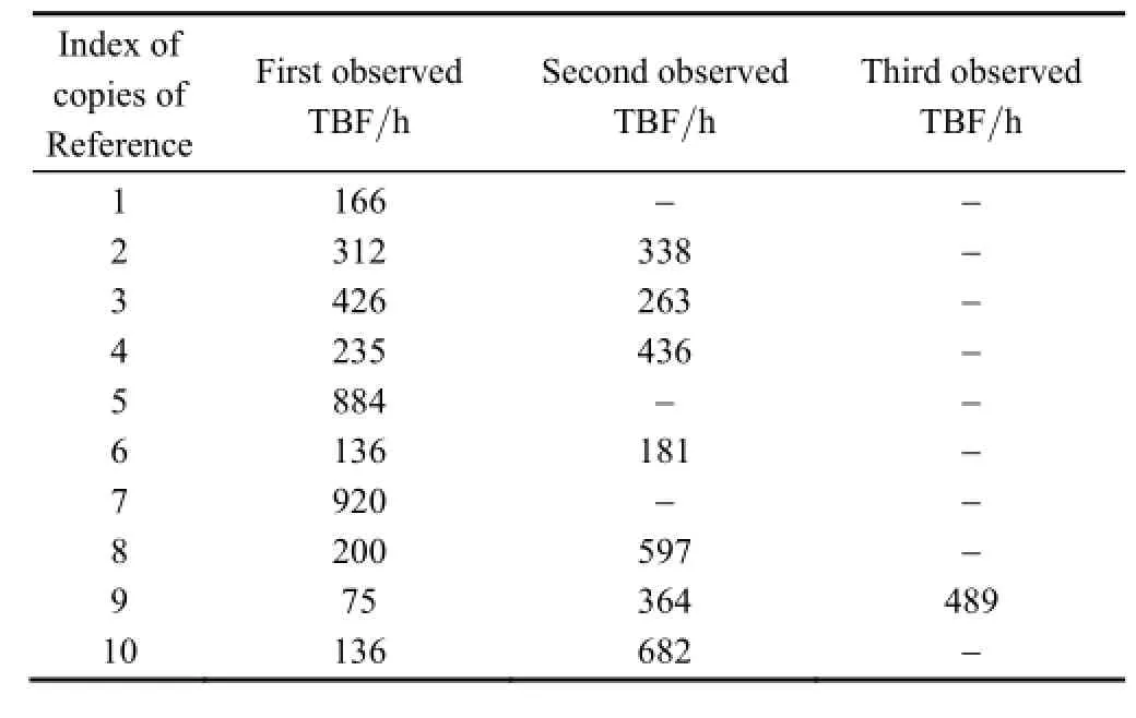
Table 2. Historical data of 10 copies of the Reference Systems

Two sets of specific questions are proposed as follows.

（1） First set of questions

Q1: For the function F0-1（P） of the Target， provide the minimum and maximum values （Lt01and Ut01） of t01at P1= 0.25.

Q2: For the function F0-1（P） of the Target， provide the minimum and maximum values （Lt02and Ut02） of t02at P2= 0.75.

（2） Second set of questions

Suppose that there are 100 similar Targets being tested under the same situation； any single Target System will be removed from the test for good after its first failure.

Q1*: How long does it take until the number of removed Target Systems reaches 25？ Provide the minimum and maximum values of this duration（Lt01and Ut01）.

Q2*: How long does it take until the number of removed Targets reaches 75？ Provide the minimum and maximum values of this duration（Lt02and Ut02）.

6.5 Expert judgments

Before answering， each expert collected and processed the multi-source prior information， and each technical expert was assigned a weight by the assessor to indicate his importance. The individual and combined answers are displayed in Table 3.

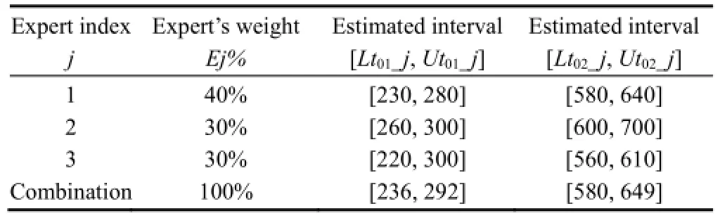
Table 3. Results of expert judgment

6.6 Calculating prior distributions

According to Table 3 and Section 2.4， the minimum and maximum values after rounding are as follows: αL=481，αU=550， βL=1.55， and βU=2.29. The prior distributions for the Target's parameters are as follows: π（α）=1/（αU-αL）=1/69， π（β）=1/（βU-βL）=1/0.74， and π（θ）=π（α）π（β）= 1/51.06， where α∈（481， 550）， β∈（1.55， 2.29）.

6.7 Calculating the posterior distributions

According to Table 1， the data sample for the Target is t=［50， 1080， 1462， 1680］.

For α， the domain ［αL， αU］=［481，550］ is divided into nα=69 sub-intervals with equal width of Δα=（αU-αL）/nα=1， and the midpoint αiin each sub-interval is selected. According to Eq. （17）， the approximate prior distribution for α is πm（αi）=1/69， and the domain is｛αi｝=｛481.5， 482.5，…， 549.5｝， i=1， 2，…， 69.

For β， the domain ［βL， βU］=［1.55， 2.29］ is divided into nβ=74 sub-intervals with equal width of Δβ=（βU-βL）/nβ=0.01， and the midpoint βjin each sub-interval is selected. According to Eq. （18）， the approximate prior distribution for β is πm（βj）=1/74， and the domain is｛βj｝=｛1.555， 1.565，…， 2.285｝， j=1， 2，…， 74.

According to Eq. （19）， the approximate prior distribution for θ is πm（θi，j）=πm（αi）πm（βj）=1/5106， and the domain is｛θi，j｝=｛（αi， βj）｝， i=1， 2，…， 69， j=1， 2，…， 74.

Given πm（αi）， πm（βj）， and t， the posterior probability at each （αi， βj） is obtained by Eq. （22）. The point estimators are obtained by Eqs. （24） and （27）. The 90% credible intervals for α and β are obtained by Eqs. （28）， （29）， （30），and （31）. These calculations were realized by a computer program， and the results are listed in Table 4.

6.8 Estimators based on an MCMC algorithm

Under the same prior distributions and data， an MCMC algorithm was developed in WinBUGS software， which does not recognize the right-hand expression of Eq. （10） as a standard Weibull PDF. Thus， the “zeros trick” that is capable of specifying a non-standard distribution was used. Ref. ［33］ introduced the “zeros trick” in detail. The Bugs code， which is the core for an MCMC algorithm in WinBUGS， is as follows:

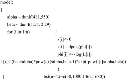
The length of the Markov chain for each parameter is10 000， and the first 500 sampled values are discarded as the burn-in. The remaining 9500 sampled values are used to calculate the estimates. The other considerations and details for this software can be found in Ref. ［33］.

6.9 Comparison of the two methods

The Bayesian point estimators and 90% credible intervals obtained by the proposed method and the MCMC algorithm are listed in Table 4. MTBF （unit: h）， an important reliability attribute of NC machine tools， can be calculated by substituting the corresponding values into α*Γ（1+1/β）， where Γ（*） is the gamma function. The MTBFs obtained by the two methods are also shown in Table 4.

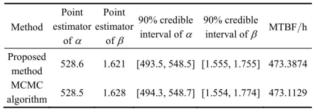
Table 4. Comparison of the proposed method and MCMC

Table 4 reveals the following.

（1） If the posterior mean values are selected as the point estimators， then the point estimators and 90% credible intervals obtained by the two methods are very close.

（2） If MTBF=473.112 9 h estimated by the MCMC algorithm is regarded as the standard， the relative error of MTBF=473.3874 h estimated by the proposed method is 5.802 0×10-4， indicating that the proposed method is as accurate as the MCMC algorithm.

（3） The pure running time consumed by the proposed programmed grid approximation method is less than 1 s. Given that the MCMC algorithm in WinBUGS involves a random-sampling process， the pure running time consumed by the MCMC simulation in WinBUGS usually costs tens of seconds.

7 Conclusions

（1） A structured process of expert judgment elicitation is designed， and expert judgments are translated into prior distributions of Weibull parameters. This method， which considers multi-source prior information， avoids the subjective bias of experts and significantly improves accuracy.

（2） High-dimensional integration in calculating the posterior is solved by grid approximation. The formulas for calculating the statistics， such as the point estimators and 90% credible intervals of the parameters， are derived.

（3） An application of the proposed method is demonstrated， and the MCMC algorithm is implemented for comparison. The results obtained by the two methods are close. The comparison indicates that the proposed method is as accurate as the MCMC algorithm.

（4） The proposed method is easier to understand and program is compared with MCMC algorithms. The convenience the proposed method provides can widen the use of Bayesian methods among engineers in the engineering field of NC machine tools who are not very good at complicated theories and lack programming skills.

References

［1］ YANG Zhaojun， CHEN Chuanhai， CHEN Fei， et al. Progress in the research of reliability technology of machine tools［J］. Journal of Mechanical Engineering， 2013， 49（20）: 130-139. （in Chinese）

［2］ KELLER A Z， KAMATH A R R， PERERA U D. Reliability analysis of CNC machine tools［J］. Reliability Engineering， 1982，3（6）: 449-473.

［3］ JIA Yazhou， WANG Molin， JIA Zhixin. Probability distribution of machining center failures［J］. Reliability Engineering and System Safety， 1995， 50（1）: 121-125.

［4］ YANG Zhaojun， CHEN Chuanhai， CHEN Fei， et al. Reliability analysis of machining center based on the field data［J］. Eksploatacja i Niezawodność， 2013， 15（2）: 147-155.

［5］ YANG Jianguo， WANG Zhiming， WANG Guoqiang， et al. Likelihood ratio test interval estimation of reliability indices for numerical control machine tools［J］. Journal of Mechanical Engineering， 2012， 48（2）: 9-15. （in Chinese）

［6］ ZHANG Genbao， TANG Xianjin， LIAO Xiaobo， et al. Quantitative modeling and application of CNC machine failure distribution curve［J］. Journal of Chongqing University， 2013， 36（6）: 119-123.（in Chinese）

［7］ CHEN Diansheng， WANG Tianmiao， WEI Hongxing. Sectional model involving two Weibull distributions for CNC lathe failure probability［J］. Journal of Beijing University of Aeronautics and Astronautics， 2005， 31（7）: 766-769. （in Chinese）

［8］ ZHANG L F， XIE M， TANG L C. Bias correction for the least squares estimator of Weibull shape parameter with complete and censored data［J］. Reliability Engineering and System Safety， 2006，91（8）: 930-939.

［9］ MONTANARI G C， MAZZANTI G， CACCIARI M， et al. In search of convenient techniques for reducing bias in the estimation of Weibull parameters for uncensored tests［J］. IEEE Transactions on Dielectrics and Electrical Insulation， 1997， 4（3）: 306-313.

［10］ FULTON J W， ABERNETHY R B. Likelihood adjustment: A simple method for better forecasting from small samples［C］// Proceedings of IEEE Annual Reliability and Maintainability Symposium， Los Angeles， CA， USA， January 24-27， 2000: 150-154.

［11］ HAMADA M S， WILSON A G， REESE C S， et al. Bayesian Reliability［M］. New York: Springer， 2008.

［12］ GUIKEMA S D， PATÉ-CORNELL M E. Bayesian analysis of launch vehicle success rates［J］. Journal of Spacecraft and Rockets，2004， 41（1）: 93-102.

［13］ GUIKEMA S D， PATÉ-CORNELL M E. Probability of infancy problems for space launch vehicles［J］. Reliability Engineering and System Safety， 2005， 87（3）: 303-314.

［14］ GUIKEMA S D. A comparison of reliability estimation methods for binary systems［J］. Reliability Engineering and System Safety， 2005，87（3）: 365-376.

［15］ ANDERSON-COOK C M， GRAVES T， HAMADA M， et al. Bayesian stockpile reliability methodology for complex systems［J］. Military Operations Research， 2007， 12（2）: 25-37.

［16］ PENG Weiwen， HUANG Hongzhong， LI Yanfeng， et al. Bayesian information fusion method for reliability assessment of milling head［J］. Journal of Mechanical Engineering， 2014， 50（6）: 185-191.（in Chinese）

［17］ MING Zhimao， ZHANG Yunan， TAO Junyong， et al. Bayesian reliability assessment and prediction during product development［J］. Journal of Mechanical Engineering， 2010， 46（4）:150-156. （in Chinese）

［18］ QUIGLEY L， BEDFORD T， WALLS L. Prior distribution elicitation， encyclopedia of statistics in quality and reliability［M］. New York: John Wiley & Sons Ltd.， 2008.

［19］ WALLS L， QUIGLEY J. Building prior distributions to support Bayesian reliability growth modelling using expert judgement［J］. Reliability Engineering and System Safety， 2001， 74（2）: 117-128.

［20］ MEYER M A， BOOKER J M. Eliciting and analyzing expert judgment: a practical guide［M］. London: Academic Press， 1991.

［21］ KAMINSKIY M P， KRIVTSOV V V. A simple procedure for Bayesian estimation of the Weibull distribution［J］. IEEE Transactions on Reliability， 2005， 54（4）: 612-616.

［22］ GARTHWAITE P H， KADANE J B， O'HAGAN A. Statistical methods for eliciting probability distributions［J］. Journal of the American Statistical Association， 2005， 100（470）: 680-701.

［23］ ALBERT I， DONNET S， GUIHENNEUC-JOUYAUX C， et al. Combining expert opinions in prior elicitation［J］. Bayesian Analysis，2012， 7（3）: 503-532.

［24］ KADANE J B， DICKEY J M， WINKLER R L， et al. Interactive elicitation of opinion for a normal linear model［J］. Journal of the American Statistical Association， 1980， 75（372）: 845-854.

［25］ LOW-CHOY S， MURRAY J， JAMES A， et al. Indirect elicitation from ecological experts: from methods and software to habitat modelling and rock-wallabies［J］. The Oxford Handbook of Applied Bayesian Analysis， 2010: 511-544.

［26］ SOLAND R M. Bayesian analysis of the Weibull process with unknown scale and shape parameters［J］. IEEE Transactions on Reliability， 1969， 18（4）: 181-184.

［27］ METROPOLIS N， ROSENBLUTH A W， ROSENBLUTH M N， et al. Equation of state calculations by fast computing machines［J］. The journal of chemical physics， 1953， 21（6）: 1087-1092.

［28］ HASTINGS W K. Monte Carlo sampling methods using Markov chains and their applications［J］. Biometrika， 1970， 57（1）: 97-109.

［29］ GELFAND A E， SMITH A F M. Sampling-based approaches to calculating marginal densities［J］. Journal of the American Statistical Association， 1990， 85（410）: 398-409.

［30］ NEAL R M. Slice sampling［J］. The Annals of Statistics， 2003， 31（3）: 705-767.

［31］ GUPTA A， MUKHERJEE B， UPADHYAY S K. Weibull extension model: A Bayes study using Markov chain Monte Carlo simulation［J］. Reliability Engineering and System Safety， 2008，93（10）: 1434-1443.

［32］ SOLIMAN A A， ABD-ELLAH A H， ABOU-ELHEGGAG N A， et al. Modified Weibull model: A Bayes study using MCMC approach based on progressive censoring data［J］. Reliability Engineering and System Safety， 2012， 100（2）: 48-57.

［33］ LUNN D， JACKSON C， BEST N. et al. The BUGS book: a practical introduction to Bayesian analysis［M］. Boca Raton: CRC Press， 2012.

［34］ KRUSCHKE J K. Doing Bayesian data analysis: A tutorial with R

［35］ O'HAGAN A， BUCK C E， DANESHKHAH A， et al. Uncertain judgements: eliciting experts' probabilities［M］. Chichester: John Wiley & Sons， Ltd.， 2006.

［36］ BERGER J O. Statistical decision theory and Bayesian analysis［M］. Berlin: Springer， 1985.

［37］ RINNE H. The Weibull distribution: a handbook［M］. Boca Raton: CRC Press， 2009.

［38］ YOUNG G A， SMITH R L. Essentials of statistical inference［M］. New York: Cambridge University Press， 2005.

［39］ ZHANG L F， XIE M， TANG L C， A study of two estimation approaches for parameters of Weibull distribution based on WPP［J］. Reliability Engineering and System Safety， 2007， 92（3）: 360-368. and BUGS［M］. Burlington: Academic Press， 2011.

Biographical notes

YANG Zhaojun， born in 1956， is currently a professor at College of Mechanical Science and Engineering， Jilin University， China. He received his PhD degree from Jilin University， China， in 1995. His research interests include reliability techniques and theories of CNC equipment.

Tel: +86-431-85095757； E-mail: yzj@jlu.edu.cn

KAN Yingnan， born in 1985， is currently a PhD candidate at College of Mechanical Science and Engineering， Jilin University，China. He received his master's degree from Jilin University，China， in 2009. His research interests include reliability modeling methods of CNC equipment and Bayesian reliability theory.

E-mail: kanyingnan@163.com

CHEN Fei， born in 1970， is currently an associate professor at College of Mechanical Science and Engineering， Jilin University，China. She received her PhD degree from Jilin University， China，in 2009. Her research interests include reliability techniques and theories of CNC equipment.

Tel: +86-431-85095839； E-mail: jluchenfei@163.com

XU Binbin， born in 1982， is currently a lecturer at Jilin University，China. She received her PhD degree from Jilin University， China，in 2011. Her research interests include reliability techniques and theories of CNC equipment.

E-mail: xubinbin@jlu.edu.cn

CHEN Chuanhai， born in 1983， is currently a lecturer at Jilin University， China. He received his PhD degree from Jilin University， China， in 2013. His research interests include reliability techniques and theories of CNC equipment.

E-mail: cchchina@foxmail.com

YANG Chuangui， born in 1987， is currently a master candidate at College of Mechanical Science and Engineering， Jilin University，China. He received his bachelor's degree from Jilin University，China， in 2012.

E-mail: ycgme@foxmail.com

10.3901/CJME.2015.0707.088， available online at www.springerlink.com； www.cjmenet.com； www.cjme.com.cn

* Corresponding author. E-mail: jluchenfei@163.com

Supported by Research on Reliability Assessment and Test Methods of Heavy Machine Tools， China（State Key Science & Technology Project High-grade NC Machine Tools and Basic Manufacturing Equipment，Grant No. 2014ZX04014-011）， Reliability Modeling of Machining Centers Considering the Cutting Loads， China（Science & Technology Development Plan for Jilin Province， Grant No. 3D513S292414）， and Graduate Innovation Fund of Jilin University， China（Grant No. 2014053）

© Chinese Mechanical Engineering Society and Springer-Verlag Berlin Heidelberg 2015

December 26， 2014； revised June 23， 2015； accepted July 7， 2015