Strict greedy design paradigm applied to the stochastic multi-armed bandit problem
2015-09-01JoeyHong
At each decision, the environment state provides the decision maker with a set of available actions from which to choose. As a result of selecting a particular action in the state, the environment generates an immediate reward for the decision maker and shifts to a different state and decision. The ultimate goal for the decision maker is to maximize the total reward after a sequence of time steps.
This paper will focus on an archetypal example of reinforcement learning, the stochastic multi-armed bandit problem. After introducing the dilemma, I will briefly cover the most common methods used to solve it, namely the UCB andεn-greedy algorithms. I will also introduce my own greedy implementation, the strict-greedy algorithm, which more tightly follows the greedy pattern in algorithm design, and show that it runs comparably to the two accepted algorithms.
1 Introduction
Reinforcement learning involves the optimization of the exploration of higher-reward options in the future based on the exploitation of knowledge of past rewards. Exploration-exploitation tradeoff is most thoroughly studied through the multi-armed bandit problem. The problem receives its name because of its application to the decisions facing a casino gambler when determining which slot machine, colloquially called “one-armed bandit,” to play.
The K-armed bandit problem consists ofKslot machines, each machine having an unknown stationary mean reward value in [0,1]. The observed reward of playing each machine is defined by the variableXi,n, where 1 ≤i≤Kis the index of the machine andn≥ 1 is the decision time step index. Successive plays of machineiyield rewards,Xi,1,Xi,2,… that are independent but distributed accordingtthe unknown mean valueμi. The problem proceeds as follows:
For each roundn=1, 2, …
1) The gambler chooses machinei∈ {1,…,K}.
2) The environment returns rewardXi,naccording to meanμibut independent of past rewards.
2 Background
A policy or allocation strategy is an approach that chooses the next machine based on the results of previous sequences of plays and rewards.
Let
or the mean value of the optimal machine.
IfTi(n) is the number of times machineihas been played, the expected loss of the policy afternplays can be written as
We also define
Lai and Robbins (1985) proved that under policies where the optimal machine is played exponentially more than sub-optimal ones, the number of plays of sub-optimal machinejis asymptotically bounded by
wheren→ ∞ and
is the Kullback-Leibler divergence between machinej’s reward densitypjand the optimal machine’sp*. Therefore, the best possible regret is shown to be logarithmic tonin behavior.
3 Algorithms
The following policies work by associating each machine with an upper confidence index. Each index acts as an estimate for the expected reward of the corresponding machine, allowing the policy to play the machine with the current highest index. We define the current average reward from machineito bewi/ni, wherewiis the total reward from machinei.
3.1 Upper confidence bounds (UCB)
The UCB policy, the most prevalent solution to the multi-armed bandit problem, is a variant of the index-based policy that achieves logarithmic regret uniformly rather than merely asymptotically. The UCB policy constructs an upper confidence bound on the mean of each arm and consequently, chooses the arm that appears most favorable under these estimates.

DeterministicPolicy:UCBInitialization:PlayeachmachineonceMain:Foreachroundn=1,2,…-Playmachinejwithmaximumxj+2lnnnjwherexjisthecurrentaveragerewardfrommachinej,njisthenumberoftimesmachinejhasbeenplayed,andnisthedecisionindexthusfar.
3.2 εn-greedy
Theεn-greedy heuristic is widely used because of its obvious generalizations to other sequential decision processes. At each time step, the policy selects the machine with the highest empirical mean value with probability 1-ε, and with probabilityε, a random machine. To keep the regret at logarithmic growth,εapproaches 0 at a rate of 1/n, wherenis still the current decision epoch index.

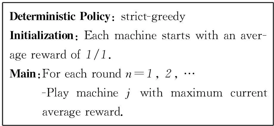
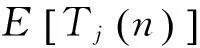
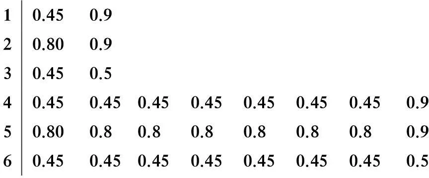
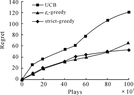
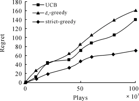
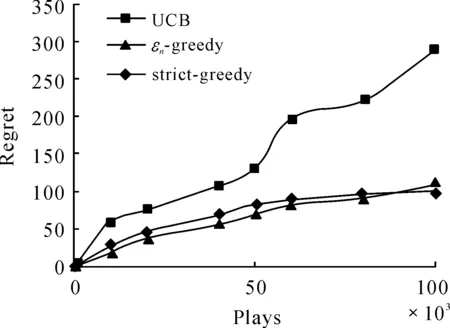
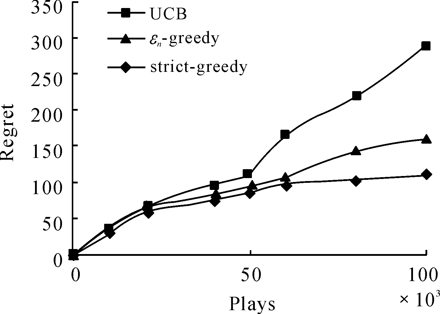
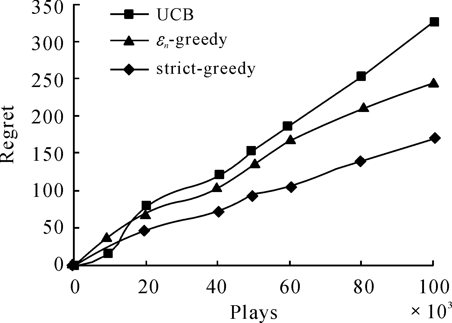
RandomizedPolicy:εn-greedy(decreasingε)Parameters:c>0and0 However, in an earlier empirical study, Vermorel and Mohri (2005) did not find any pragmatic advantages to obtaining logarithmic instead of linear bound through decreasingεover time. Our implementation will only consider fixed values ofε. The fixed ε creates a weighted equilibrium between exploration and exploitation throughout the heuristic. RandomizedPolicy:εn-greedy(fixedε)Parameters:0<ε<1.Initialization:PlayeachmachineonceMain:Foreachroundn=1,2,…-Letjbethemachinewithmaximumcur-rentaveragereward-Playmachinejwithprobability1-εandarandommachinewithprobabilityε. The greedy design paradigm can be summarized as iteratively making myopic and irrevocable decisions, thereby always making the locally optimal choice in hopes of global optimum. Though the relative correctness of theεn-greedy heuristic is experimentally supported, there are several areas where it strays from the described pure greedy paradigm: 1) After the initialization where each machine is played, the greedy algorithm’s decisions are no longer parochial in nature, as the algorithm is unfairly given a broader knowledge of each machine when making decisions. Employing such initialization also requires unreasonably many steps. 2) Theεfactor in making decisions allows the algorithm to not always choose the local optimum. The introduction of randomization into the algorithm effectively disrupts the greedy design paradigm. The primary problem we face when designing the strictly greedy algorithm is in its initialization, as the absence of any preliminary knowledge of reward distributions mistakenly puts each machine on equal confidence indices. 4.1 Strict-greedy To solve the aforementioned dilemma, each machine is initialized with average reward 1/1. Therefore, each machine can be effectively played until its return drops below 1, where the algorithm deems the machine inadequate and moves to another machine. The capriciousness of the policy allows the optimal machine to be quickly found, and thus, likely minimizes the time spent on suboptimal states. The policy, therefore, encourages explorative behavior in the beginning and highly exploitative behavior towards the end. However, this policy’s behavior also does not exhibit uniform or asymptotic logarithmic regret. DeterministicPolicy:strict-greedyInitialization:Eachmachinestartswithanaver-agerewardof1/1.Main:Foreachroundn=1,2,…-Playmachinejwithmaximumcurrentaveragereward. 4.2 Proof The following proof is inspired from the proof of the aboveεn-greedy heuristic shown in “Finite-time Analysis of the Multiarmed Bandit Problem.” Claim.We denoteItas the machine played at playt, so which isthe sum of probabilities playtresults in suboptimal machinej. The probability that strict-greedy chooses a suboptimal machine is at most whereΔj=μ*-μj and Proof. Recall that because analysis is same for both terms on the right. By Lemma 1 (Chernoff-Hoeffding Bound), we get Since we have that where in the last line, we dropped the conditional term because machines are played independently of previous choices of the policy. Finally, which concludes the proof. Each policy was implemented with a maximum heap data structure, which used a Boolean operator to choose the higher average reward or UCB index. If ties exist, the operator chooses the machine that has been played more often, and after that, randomly. Because of the heap’s logarithmic time complexities in insertions and constant time in extracting maximums, the bigOnotation for each algorithm’s runtime isO(K+nlogK) for UCB andεn-greedy andO(nlogK) for the strict-greedy, where n is the total rounds played andKis the number of slot machines, revealing a runtime benefit for the strict-greedy for largeK. In the implementation of theεn-greedy strategy,εwas arbitrarily assigned the value 0.01, to limit growing regret while ensuring a uniform exploration. A finite-time analysis of the 3 specified policies on various reward distributions was used to assess each policy’s empirical behavior. The reward distributions are shown in the following table: 10.450.920.800.930.450.540.450.450.450.450.450.450.450.950.800.80.80.80.80.80.80.960.450.450.450.450.450.450.450.5 Note that distributions 1 and 4 have high variance with a highμ*, distributions 2 and 5 have low variance with highμ*, and distribution 3 and 6 have low variance with lowμ*Distributions 1-3 are also 2-armed variations whereas distributions 4-6 are 8-armed. In each experiment, we tracked the regret, the difference between the reward of always playing the optimal machine and the actual reward. Runs on the plots (shown in next page) were done in a spread of values from 10 000 to 100 000 plays to keep runtime feasible. Each point on the plots is based on the average reward calculated from 50 runs, to balance out the effects of anomalous results. Fig.1 shows that the strict-greedy policy runs better than the UCB policy for smallx, but falls in accuracy at 100 000 plays due to its linear regret, which agrees with the earlier proof. Theεn-greedy preforms always slightly worse, but that may be attributed to a suboptimally chosen parameter, which increases its linear regret growth. Fig.1 Comparison of policies for distribution 1 (0.45, 0.9) Fig.2 shows that all 3 policies lose accuracy in “harder” distributions (smaller variances in reward distributions). The effect is more drastically shown for smaller number of plays, as it merely takes longer for each policy to find the optimal machine. Fig.3 reveals a major disadvantage of the strict-greedy, which occurs whenμ*is small. The problem arises because the optimal machine does not win most of its games, or significantly more games than the suboptimal machine, due to its small average reward, rendering the policy less able to find the optimal machine. This causes the strict-greedy to degrade rapidly, more so than an inappropriately tunedεn-greedy heuristic. Fig.2 Comparison of policies for distribution 2 (0.8, 0.9) Fig.3 Comparison of policies for distribution 3 (0.45, 0.5) Fig.4 and Fig.5 reveal the policies under more machines. Theεn-greedy algorithm is more harmed by the increase in machines, as it uniformly explores all arms due to its randomized nature. The suboptimal parameter for theεn-greedy algorithm also causes the regret to grow linearly with a larger leading coefficient. The strict-greedy policy preforms similarly to, if not better than, the UCB policy for smaller number of plays even with the increase in number of machines. Fig.6 reaffirms the degrading strict-greedy policy whenμ*is small. The linear nature of the strict-greedy is most evident in this case, maintaining a relatively steady linear regret growth. However, the policy still preforms better than theεn-greedy heuristic. Fig.4 Comparison of policies for distribution 4 (0.45, 0.45, 0.45, 0.45, 0.45, 0.45, 0.45, 0.9) Fig.5 Comparison of policies for distribution 5 (0.8, 0.8, 0.8, 0.8, 0.8, 0.8, 0.8, 0.9) Fig.6 Comparison of policies for distribution 6 (0.45, 0.45, 0.45, 0.45, 0.45, 0.45, 0.45, 0.5) The comparison of all the policies can be summarized in the following statements (see Figures 1-6 above): 1) The UCBand strict-greedy policies preform almost always the best, but for large number of plays, the strict-greedy falls because of its linear, not logarithmic, regret. Theεn-greedy heuristic preforms almost always the worst, though this can be due to a suboptimally tuned parameter. 2) All 3 policies are harmed by an increase in variance in reward distributions, butεn-greedy degrades most rapidly (especially when there are a lot of suboptimal machines) in that situation because it explores uniformly over all machines. 3) The strict-greedy policy undergoes weak performance whenμ*is small, because its deterministic greedy nature makes it more difficult to play the optimal arm when its reward is not significantly high. 4) Of the 3 policies, the UCB showed the most consistent results over the various distributions, or least sensitive to changes in the distribution. We have analyzed simple and efficient policies for solving the multi-armed bandit problem, as well as introduced our own deterministic policy, also based on an upper confidence index. This new policy is more computationally efficient than the other two, and runs comparably well, but still proves less reliable than the UCB solution and is unable to maintain optimal logarithmic regret. Due to its strict adherence to the greedy pattern, it can be generalized to solve similar problems that require the greedy design paradigm. References [1]Auer P,Cesa-Bianchi N, Fischer P. Finite-time Analysis of the Multiarmed Bandit Problem[J]. Machine Learning, 2002,47. [2]Bubeck S,Cesa-Bianchi N.Regret Analysis of Stochastic and Nonstochastic Multi-armed Bandit Problems[J]. 2012. [3]Kuleshov V,Precup D.Algorithms for the multi-armed bandit problem[Z]. [4]Puterman M.Markov Decision Processes: Discrete Stochastic Dynamic Programming[M].USA:John Wiley & Sons Inc,2005. 16 August 2014; revised 12 October 2014;accepted 25 September 2014 Strict greedy design paradigm applied to the stochastic multi-armed bandit problem Joey Hong (TheKing’sAcademy,Sunnyvale,CA) The process of making decisions is something humans do inherently and routinely, to the extent that it appears commonplace. However, in order to achieve good overall performance, decisions must take into account both the outcomes of past decisions and opportunities of future ones. Reinforcement learning, which is fundamental to sequential decision-making, consists of the following components: ① A set of decisions epochs; ② A set of environment states; ③ A set of available actions to transition states; ④ State-action dependent immediate rewards for each action. Greedy algorithms, Allocation strategy, Stochastic multi-armed bandit problem TP18 10.3969/j.issn.1001-3881.2015.06.001 Document code: A *Corresponding author: Joey Hong,E-mail:jxihong@gmail.com Hydromechatronics Engineering http://jdy.qks.cqut.edu.cn E-mail: jdygcyw@126.com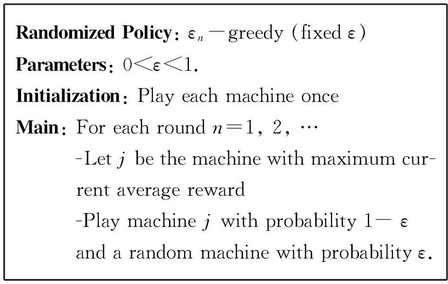
4 A pure greedy algorithm

5 Experimentation

6 Conclusions
杂志排行

机床与液压的其它文章
- Research on comprehensive index system about product quality monitoring
- Exploration on the calculating formula of main transmission chain structural formulas of machine tools
- Visualization study of the oscillating bubble near the elastic wall
- Study on electro-hydraulic load simulator based on flow compensation method
- Optimal design for amplifier of jet deflector servo valve
- Availability function deployment of the CNC lathe based on multi factors