Numerical simulation unsteady cloud cavitating flow with a filter-based density correction model*
2014-06-01HUANGBiao黄彪WANGGuoyu王国玉ZHAOYu赵宇
HUANG Biao (黄彪), WANG Guo-yu (王国玉), ZHAO Yu (赵宇)
School of Mechanics and Engineering, Beijing Institute of Technology, Beijing 100081, China, E-mail: huangbiao@bit.edu.cn
Numerical simulation unsteady cloud cavitating flow with a filter-based density correction model*
HUANG Biao (黄彪), WANG Guo-yu (王国玉), ZHAO Yu (赵宇)
School of Mechanics and Engineering, Beijing Institute of Technology, Beijing 100081, China, E-mail: huangbiao@bit.edu.cn
(Received September 19, 2012, Revised November 20, 2012)
In this paper, various turbulence closure models for unsteady cavitating flows are investigated. The filter-based model (FBM) and the density correction model (DCM) were proposed to reduce the turbulent eddy viscosities in a turbulent cavitating flow based on the local meshing resolution and the local fluid density, respectively. The effects of the resolution control parameters in the FBM and DCM models are discussed. It is shown that the eddy viscosity near the cavity closure region can significantly influence the cavity shapes and the unsteady shedding pattern of the cavitating flows. To improve the predictions, a Filter-Based Density Correction model (FBDCM) is proposed, which blends the FBM and DCM models according to the local fluid density. The new FBDCM model can effectively represent the eddy viscosity, according to the multi-phase characteristics of the unsteady cavitating flows. The experimental validations regarding the force analysis and the unsteady cavity visualization show that good agreements with experimental visualizations and measurements are obtained by the FBDCM model. For the FBDCM model, the attached cavity length and the resulting hydrodynamic characteristics are subsequently affected by the detail turbulence modeling parameters, and the model is shown to be effective in improving the overall predictive capability.
CFD, cavitating flows, resolution control parameter, turbulence model
Introduction
The cavitation plays an important role in the design and operation of fluid machinery and devices because it causes performance degradation, noise, vibration, and erosion. The cavitation involves complex phase-change dynamics, large density ratio between phases, and multiple time scales. The homogeneous two-phase Navier-Stokes equations were successfully applied for the simulations of cavitating flows[1]. The accuracy, stability, efficiency and robustness of the modeling strategies are a big challenge because of the complex interactions associated with unsteady turbulent cavitating flows.
The turbulence closure model plays a very significant role in the simulations of the cavitating flows, with typically a high Reynolds number and with mass transfer between a two phase medium. The Reynoldsaveraged Navier-Stokes (RANS) turbulence models, such as the originalkε- model, were initially developed for fully incompressible fluids. Hence, they are not suitable for highly compressible two-phase mixture flows, which is why they were found to be unsatisfactory for predicting cavitating flows with high compressibility in the vapor region. The re-entrant jet instability is often attributed to the cavity destabilization and the transition to the unsteady cavitation. In experiments, it was demonstrated that the re-entrant jet in the closure region is the basic mechanism that triggers the break up and shedding of unsteady cavity clouds[2,3]. To account for the large density jump caused by cavitation and re-entrant jet near the closure region, Coutier-Delgosha et al.[4]modified the turbulent viscosity to simulate the cloud cavity shedding in a Venturi-type duct. They found that the influence of the compressibility of the two-phase medium was significant in simulating the turbulence effects on the cavitating flow. The modified turbulent viscosity model could predict the unsteady re-entrant jet and the shedding of the vapor cloud, but the length and the shedding frequency were not accurately predicted for cases with high cavitation numbers. This is due to thefact that the Coutier-Delgosha’s turbulence modification can not completely account for all complex flow features present in the cavity closure region. Recently, to capture the unsteady characteristics between the quasi-periodic large-scale and turbulent small-scale features of the flow field, a large eddy simulation (LES) model was used to simulate the sheet/cloud cavitation on a NACA0015 hydrofoil[5]. However, it is fundamentally difficult to find a grid independent LES solution unless one explicitly assigns a filter scale. Moreover, the computational cost of the LES is very high. The very large eddy simulation (VLES) attempts to strike a compromise between the RANS and the LES. The detached eddy simulation (DES) was widely used as a modified hybrid RANS-LES approach. Huang et al.[6]evaluated an enhanced turbulence modeling scheme based on the DES, the results showed that a standard RANS model fails to predict marginally the stable cavities whereas the DES model appeared to provide more accurate flow modeling, possibly because the DES can better handle the large scale closure dynamics. Johansen et al.[7]formulated a filterbased model (FBM) to avoid some of the known deficiencies of the RANS approaches, and the difficulties in the application of the LES. Wu et al.[8]assessed the validity of FBM turbulence models through unsteady simulations of different geometries, including a square cylinder, a convergent-divergent nozzle, a Clark-Y hydrofoil, and a hollow-jet valve. They found that the FBM can better capture the unsteady features, and yield a stronger time-dependency in the cavitating flows, than the originalkε- model. Kim and Brewton[9]compared the numerical predictions with RANS, LES, and RANS/LES hybrid approaches for the sheet/cloud cavitation, the LES and the RANS/ LES hybrid results closely reproduced the salient features such as the breakup of the sheet cavity by a reentrant jet, and the formation and collapse of the cloud cavity.
Previous researches showed that the adopted turbulence model has a strong effect on the predicted cavity shape and stabilities[4,9]. The physical mechanisms are not well understood due to the complex cavitating flow structures. Hence, better modeling approaches are highly in demand. In the following sections, differentkε- based turbulence models from the literature are summarized followed by an introduction of a filter-based density corrected model (FBDCM) based on the unsteady characteristics of the cavitating flow. The objective of this paper is to present a new FBDCM for improving the numerical predictions of turbulent cavitating flows, and to investigate the accuracy and stability of various turbulent closure models for the unsteady cavitating flows by comparing the numerical predictions with experimental measurements.
1. Numerical model in cavitation computation
1.1Continuity and momentum equations
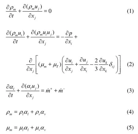
The Navier-Stokes equations for a Newtonian fluid without body forces and heat transfers, in their conservative form, in the Cartesian coordinates, are as follows: whereρmis the mixture density,ρlis the liquid density,ρvis the vapor density,αvis the vapor fraction,αlis the liquid fraction,uis the velocity,pis the pressure,μmis the mixture laminar viscosity,μlandμvare the liquid and vapor laminar viscosities,μTis the turbulent viscosity. The subscripts (i,j,k) denote the components related to the appropriate Cartesian coordinates. The source termm˙+, and the sink termm˙-, in Eq.(3) represent the condensation and evaporation rates, respectively. In the present study, the phenomenological Kubota cavity transport model is used:
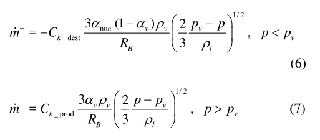
wherenuc.αis the nucleation volume fraction,BRis the bubble diameter,vpis the saturated liquid vapor pressure, andpis the local fluid pressure.destCis the rate constant for the vapor generated from the liquid ina region where the local pressure is less than the vapor pressure. Conversely,Cprodis the rate constant for reconversion of the vapor back into the liquid in the regions where the local pressure exceeds the vapor pressure. As shown in Eqs.(6) and (7), both the evaporation and condensation terms are assumed to be proportional to the square root of the difference between the local pressure and the vapor pressure. In this work, the assumed values for the model constants areαnuc.=5× 10⁻⁴,RB=1×10⁻⁶m,Cdest=50 andCprod=0.01.
1.2Summary ofkε--based turbulence model
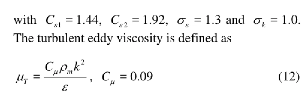
Thekε- andkω- turbulence models are the most commonly used of all two-equation turbulence models. The primary disadvantage of thekω- model, in its original form, is that boundary layer computations are very sensitive to the values of the vorticityωin the free stream. In the case of unsteady cavitating flows, this sensitivity might cause inaccurate predictions of the fluid physics.
1.2.1 Model-1: Originalkε- turbulence model
The originalkε- turbulence model falls within this class of turbulence models and has been the workhorse of practical engineering flow calculations since it was proposed by Launder and Spalding. The benefit of thekε- model is that it is not as sensitive to the free streamω,s in thekω- model. Thekεmodel includes two partial differential equations for the transport of the turbulent kinetic energykand the dissipation rateε:

The originalkε- model was originally developed for fully incompressible single phase flows, and was not intended for flow problems involving highly compressible multiphase mixtures. Previous researches[4]show that the two-equation model over-predicts the turbulence kinetic energy, and hence the turbulent viscosity, which results in an over-prediction of the turbulent stresses, causing the reentrant jet in the cavitating flows to lose momentum. Thus, the re-entrant jet can not cut across the cavity sheet, which significantly modifies the cavity shedding behavior.
Hence, a systematic method to lower the turbulent viscosity in the vapor region is necessary to improve the prediction of the reentrant jet and the vapor dynamics in unsteady cavitating flows.
1.2.2 Model-2: Filter-based turbulence model (FBM)
(from Refs.[7])
Johansen et al.[7]proposed a special filter to help reduceTμ, if the turbulent scales are smaller than a set filter size, they will not be resolved. Specifically, the level of the turbulent viscosity is corrected by comparing the turbulence length scale and the filter sizeλ, which is selected based on the local meshing spacing

1.2.3 Model-3: Density corrected model (DCM) (from Refs.[4])
To improve numerical simulations by taking into account the influence of the compressibility of the two-phase mediums on the turbulence, Coutier-Delgosha et al.[4]proposed to reduce the mixture turbulent viscosity based on the local liquid volume fractionlα:

In the above equations, all the parameters, except for the functionDCMf, are set to the values originally proposed by Launder and Spalding.
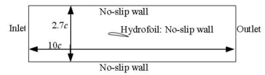
Fig.1 Boundary conditions for Clark-Y hydrofoil
The capabilities for simulating unsteady cavitating flows of the different models are further investigated. The computational domain with 42 000 cells and boundary conditions are considered according to the experimental setup in Ref.[10], as shown in Fig.1. A no-slip boundary condition is imposed on the hydrofoil surface, and no-slip symmetry conditions are imposed on the top and bottom boundaries of the tunnel. The foil has a uniform cross-section with an Clark-Y thickness distribution with a maximum thickness-to-chord ratio of 12%, the Clark-Y foil is located at the center of the test section with the angle of attack of 8o, and the chord length of the hydrofoil is =c0.07 m, and the span length is =s0.07 m. The two important dimensionless parameters are the Reynolds numberReand the cavitation numberσ, the saturated vapor pressurevp, and the inlet velocityU∞are expressed as in Eq.(15). Computations are made for the cloud cavitation condition (σ=0.8), and the outlet pressure is set to vary according to the cavitation number. A constant velocity is imposed at the inlet,U∞=10 m/s, with the corresponding Reynolds number ofRe=7×10⁵. The density and the dynamic viscosity of the liquid are taken to beρl=999.19 kg/m3andμl=ρlvl=1.139× 10–3Pa·s, respectively, for fresh water at 25oC. The vapor density isρv=0.02308 kg/m3and the vapor viscosity isμv=9.8626×10⁻⁶Pa·s. The vapor pressure of water at 25oC ispv=3 169 Pa.

Based on the eddy-to-laminar viscosity ratio at the inlet,μT/μL|inlet, the inlet turbulent quantities can be computed as follows
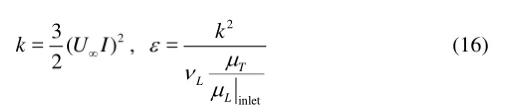
whereIis the inlet turbulence intensity, which is set to 0.02, according to the experiment[1].
2. Results and discussions
2.1Effect of FBM resolution control parameter (the filter size λ)
The general strategy of the FBM model is to limit the influence of the eddy viscosity based on the local numerical resolution. In the FBM model, the level of the turbulent viscosity is corrected by comparing the turbulence scalek3/2/εand the filter sizeλ, based on the local meshing spacing. The filter size Δ can be considered as the resolution control parameter. The value of this parameter depends on the desire physical resolution and the numerical cost associated with it.
To investigate the sensitivity of the solution to the value of the filter size, four filter sizes are examined here: 10Δgrid,maxo, 3.23Δgrid,maxo, 1.61Δgrid,maxo, and 1.05Δgrid,maxo. Here, Δgrid,maxois the largest grid size of theOshape grid around the hydrofoil in the computation domain, which is around 0.012c.
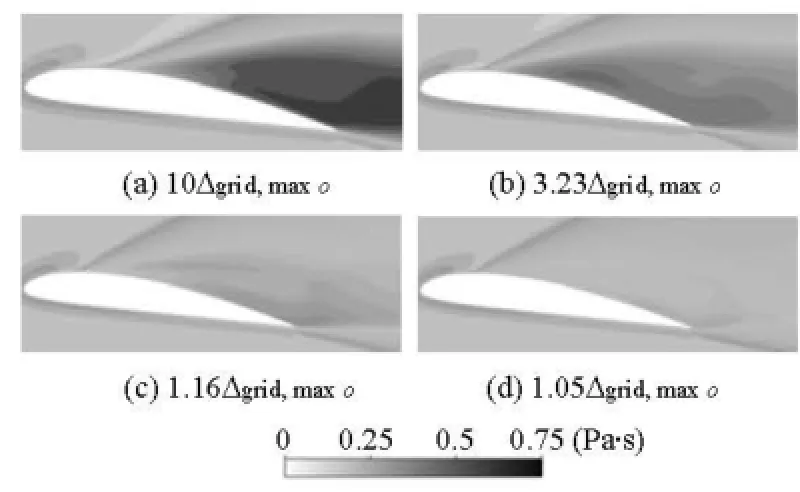
Fig.2 Time-averaged_FBMTμ contours for different filter sizes λ for the FBM model
It is immediately evident from Eq.(13) that reducing Δ leads to a linear decrease ofμT. For a largerλ,fFBMis limited to 1 because the simulation is expected to filter out most of the excessive eddy viscosity, resulting in a reduced unsteadiness of the computed flow field. However, the FBM strongly relies on the DNS on the grid resolution, as shown in Figs.2(a) and 2(d), due to the intrinsic dependence ofμTFBMon the grid size.
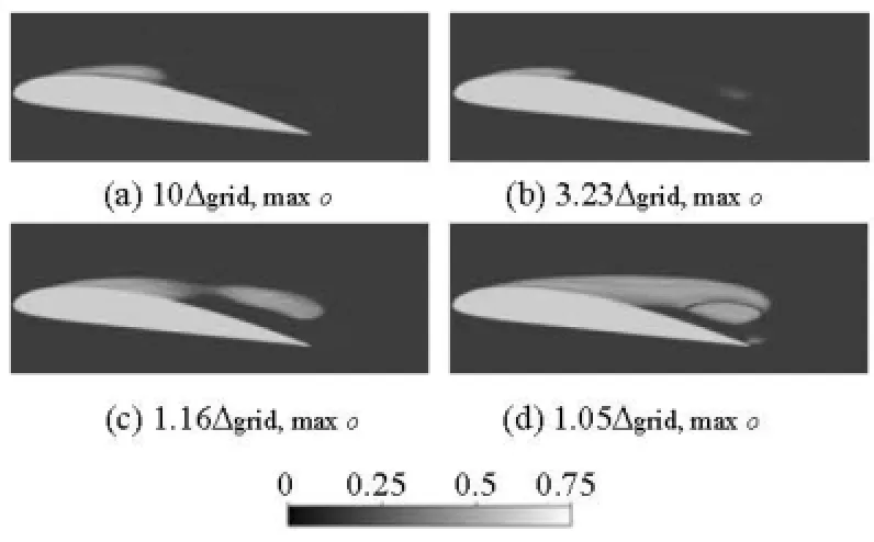
Fig.3 Time-averaged streamlines and vapor fraction for different filter sizes λ for the FBM model (=σ0.8, =Re 7×10⁵, =α8o)
Figure 3 shows the time-averaged streamlines and vapor fraction contours. It is clear that the filter size Δ has a significant impact on the time-averaged cavity patterns.
(1) The visualizations of the time-averaged cavity show very similar pictures when the filter sizes are large (such as 10Δgrid,maxo, 3.23Δgrid,maxo), where the numerical predictions fail to simulate the detached cavity near the trailing edge.
(2) As the filter size decreases, the time-averaged cavity size increases. For Δ=1.61Δgrid,maxoand Δ= 1.05Δgrid,maxo, the cavitation structures consist of two parts, an attached cavity at the leading edge and a detached cavity near the trailing edge, which is formed because the re-entrant jet is not impeded by the excessively highμT.
In order to compare the space-time evolution of the cavity shapes predicted by different schemes, the vapor volume fractions of the cavity are plotted against the time and space. Figure 4 shows comparisons between the shedding processes predicted by the FBM model of different filter sizes. In Fig.4,TrefandLrefare defined as
wherecis the chord length andU∞is the free stream velocity.ref/=x L0 corresponds to the foil leading edge, andref/=x L1.0 corresponds to the foil trailing edge. The Strouhal numbercStcharacterizing the shedding frequency can be defined as
As seen from Fig.4, the transient evolutions are almost all periodic. One may focus on details of the fluctuation period for different filter sizes in the case of the cloud cavitation:
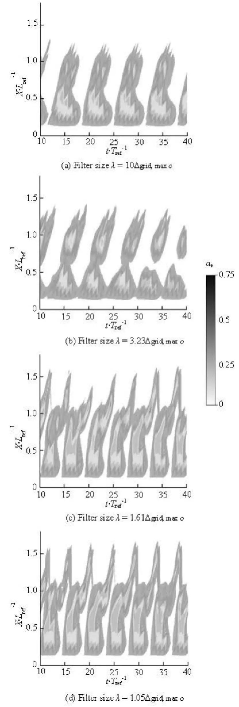
Fig.4 Time evolution of the water vapor fraction in various sections for different filter sizes λ for the FBM Model (=σ0.8, =Re7×105, =α8o)
(1) Forλ=10Δgrid,maxoandλ=3.23Δgrid,maxoas shown in Figs.4(a) and 4(b), respectively, the mean fluctuation periods are approximately 7.0Trefand 6.2Tref, respectively. The correspondingStcare 0.14 and 0.16, respectively, which are low compared to the experimentally measured value ofStc=0.18[10].
(2) Forλ=1.61Δgrid,maxoandλ=1.05Δgrid,maxo, the maximum attached cavity reaches a slightly large length of more than 1.1c, which is substantially greater than that predicted for the highλvalues. With the smaller filter size, the FBM model gradually weakens the turbulent dissipation so that the detached cavities are well captured. The Strouhal numbers predicted for the cases ofλ=1.61Δgrid,maxoandλ=1.05Δgrid,maxoseem almost the same, they are both approximately 0.185, as in good agreement with the experimental measurements.
2.2Effect of DCM resolution control parameter (the
parameter n)
The originalk-εmodel was intended for fully incompressible flows. To simulate a multiphase flow where the local compressibility near the cavity collapse region is important, the turbulent viscosity can be corrected using the DCM model as shown in Eq.(14).
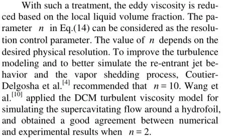
In the general scheme of the DCM model, the mixture density can be corrected byρm1=ρv+(αl)n· (ρl-ρv).The time-averaged modified density contours for different values of the parameternin the DCM model are shown in Fig.5. For the DCM model, generally speaking, the density correction function has a significant impact onμTin the cavitation region near the wall, and it has no influence in the region away from the cavity because there is no phase change. The DCM directly makes an aggressive nonlinear reduction ofμT, while the FBM makes a minor linear reduction of the eddy viscosity in the detached cavity region.
For the DCM model, the value ofnhas a significant influence on the time-averaged cavity shapes. Forn=10 andn=20, the smaller eddy viscosity, which covers entire cavity region in Figs.5(b) and 5(c) will lead to an easier cavitation.
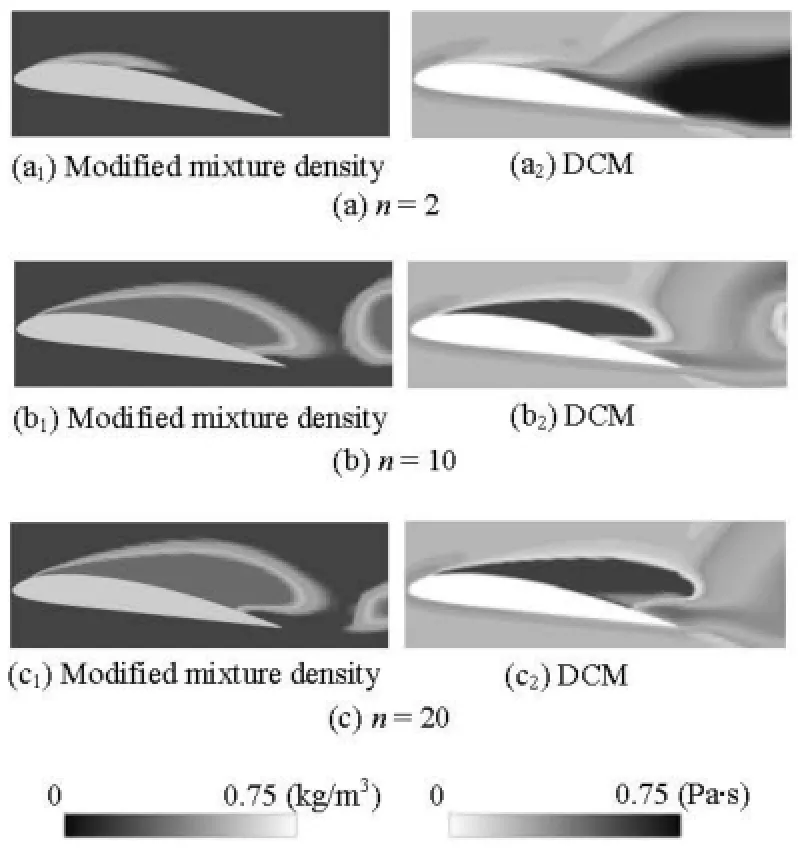
Fig.5 Time-averaged modified variable contours for different n values for the DCM model (=σ0.8, =Re7×105, =α 8o)
Figure 6 compares the shedding processes predicted by the DCM model for different values ofn, with focus on the details of fluctuation periods of cavity shapes and re-entrant flows.
(1) As shown in Fig.6, for the case ofn=2, the mean fluctuation period is about 6.8Tref, and the corresponding Strouhal number is equal to 0.145, which is lower than the measured value of 0.18. On the other hand, the Strouhal numbers predicted whenn=10 andn=20 are about 0.185, in agreement with the measured value.

2.3Introduction of a filter-based density correct
model (FBDCM) for cavitating flows
The mathematical differences in the FBM and DCM approaches lead to a major difference in the modeling results. The FBM does not correct the eddy viscosity directly near the near-wall region. As for thedensity correction function, generally speaking, it has no influence in the region away from the cavity since there is no phase change, an excessiveTμis still possible in the region surrounding the cavity.
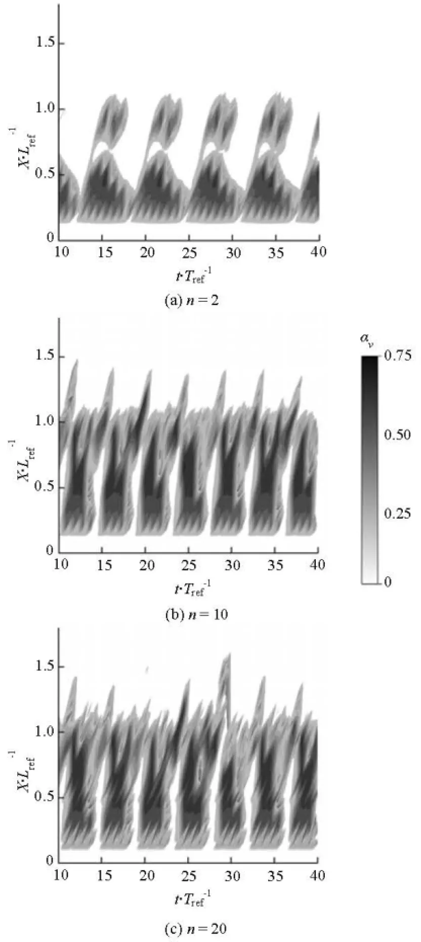
Fig.6 Time evolution of the water vapor in various sections with different values of n for the DCM model (=σ 0.8, =Re7×105, =α8o)
Considering the unsteady flow characteristics of the cavitation around the hydrofoil, the cavitation area around the hydrofoil can be divided into two sub-areas, those with attached and detached cavity, respectively[12]. The attached cavity is located in the leading edge of the hydrofoil with a relatively higher vapor volume fraction. In this region, the compressibility of the two-phase flow must be considered. While, the detached cavity contains the large-scale unsteady motion of the liquid-vapor mixture, and the local turbulent structures should be taken into account in this region.
It is clear that different models should be applied to amend the turbulent viscosity in different regions. Here, a hybrid turbulence model that combines the strengths of the FBM and DCM models is proposed below:
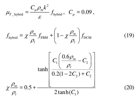
whereχ(ρm/ρl) is the hybrid function which continuously blends the FBM and DCM approaches.C1is chosen to be 4. An analysis of the hybrid model can indentify a favorable value ofC2, which regulates the affected region between the FBM model and the DCM model. Figure 7 shows the distribution of the hybrid function for the cases whenC2is equal to 0.1, 0.2, 0.3, respectively. In the FBDCM model, the filter sizeλin Eq.(9) is chosen to be 1.05Δgrid,maxo., and the parameternis chosen to be 10.
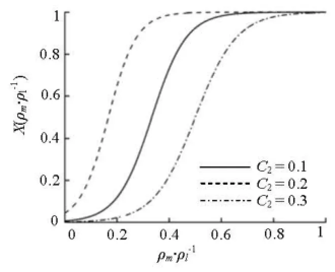
Fig.7 Distribution of hybrid function χ with different values of2C for the new hybrid FBDCM model
In order to study the differences and similarities of the resolution between different turbulence models, the time evolutions of the eddy viscosity distributions are compared. The temporal snapshots ofμTcounters are shown in Fig.8. Among the CFD results, theμTd istribu tions a re pl aced s ide by sid e according to 20%,50%,70%,and90%ofeachcorrespondingcycle. As is well known, the originalkε- model fails to reproduce the unsteady cavity development because this model yields a consistently higher eddy viscosity, resulting in a reduced unsteadiness of the computed flow field. For the FBM in Fig.8(b), based on an imposed filter, the conditional averaging is adopted for the Navies-Stokes equation to introduce one more parameter into the definition of the eddy viscosity. For the DCM in Fig.8(c), the eddy viscosity decreases intensively in the high vapor fraction areas. Although the calculated results take account of the interaction between the vapor and the mixtures, the inadequacy of the DCM under-predicts the turbulent viscosity of the tail. Compared with the simulated results with the DCM, it is clear that the FBM yields consistently a higher eddy viscosity in the recirculation region. But this model does not take into account the density fluctuations and compressibility effects in the attached cavity. As shown in FigS.8 (d)-8(e), the new FBDCM model combines the advantages of the DCM and the FBM. This new model can effectively modulate the eddy viscosity, around the leading edge of the hydrofoil, where the eddy viscosity of the DCM is used, to obtain a relatively lower density. The FBM is chosen around the rear of the hydrofoil, and produces much better resolution in capturing the unsteady features. In the FBDCM model, the value of2Ccan adjust the proportion between the FBM and DCM models in the flow field calculations.
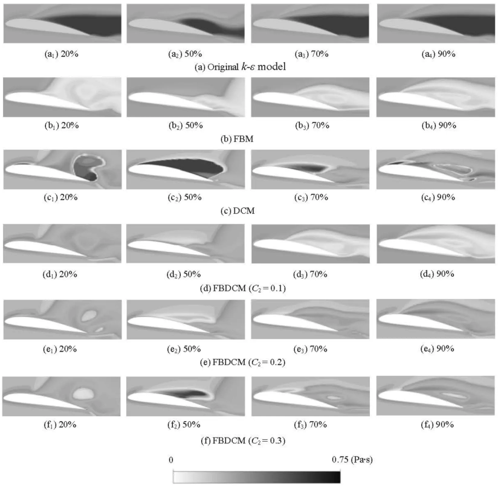
Fig.8 Time evolution ofTμ contours for different turbulence models (=σ0.8, =Re7×105, =α8o)
The differentTμdistributions will lead to diffe- rent cavity shapes, particularly, in the cavity closure region. The temporal evolutions of the cavity shapes around the hydrofoil under the cloud cavitation condition are shown in Fig.9 along with experimental observations. In experiments, the development of the cavitation can be divided into two stages: the first stage is the growth of the attached cavity immediately after a vortex shedding event, and the second stage is the detachment of the cavity due to the re-entrant flow and it overlapswith the recirculation zone near the trailing edge. The cloud cavitation predicted shows a self-oscillatory behavior characterized by sheddings of large vapor clouds, and the cavity exhibits a pronounced periodic size variation.
As the results, the originalkε- model can not capture the detached cavity during 90% of the cycle. As for the attached cavity, the maximum cavity length is no more than 50%c. For the other models, the features of every stage in experiments can be well-captured, including the detached cavity in the trailing edge, which is more consistent to the experimental observations. Although all the turbulence models predict an unstable cavity expanding and shrinking, some differences are noticeable: a bigger cavity size and a longer attached cavity length are predicted with the DCM, especially, after the cavity length reaches its maximum. The general trends for differentC2values for the FBDCM model are summarized below:
(1) Bigger cavity sizes are predicted forC2=0.3, especially, after the cavity length reaches its maximum. This is because the hybrid function of the FBDCM tends to use more portion from the DCM model forC2=0.3.
(2) During 70% and 90% of the cycle, the largescale detached cavity shedding on the rear part of the sheet cavity is captured asC2=0.1 and 0.2, but notC2=0.3.

Fig.9 Time evolution of cloud cavitation for different turbulence models (=σ0.8, =Re7×105, =α8o)
Time evolutions of the attached cavity length predicted by the hybrid model with different2Cvalues and experimental data are shown in Fig.10(a). In the numerical simulations,αl=0.9 is defined as the attached cavity boundary. The cavity lengthlis made non-dimensional by the chord lengthc. In the first stage, the length of the attached cavity increases linearly with the time. Although the comparisons of the numerical results with experimental data show that the trend is captured reasonably well for all threeC2values, the case ofC2=0.2 is compared best with the experimental data. At beginning of the second stage, a recirculation zone will include a re-entrant flow in the lower part, and the front of the re-entrant jet can be used to determine the cavity detachment point. The development of the re-entrant flow in Fig.10(b) also shows a noticeable agreement between the numerical and experimental results forC2=0.2.

Fig.10 Time evolutions of the attached cavity length and the development of the reverse flow for different values of C2for the FBDCM model (σ=0.8, Re=7×10⁵, α=8o)
From the above discussions, the features of cavity shapes and the dynamic behaviors are highly inter-related. The agreements between the CFD and the experimental data in terms of frequency are good except the originalkε- model, as shown in Table 1. One can see clearly in the case of thekε- model, there is a clear dominant frequency according to the lift history, while a lower frequency as compared with the experimental data is obtained. The frequencies are almost the same for the FBM and FBDCM models, which is because the re-entrant jet, which triggers the shedding and unsteady motion, basically consists of a high liquid volume fraction, and the FBM is more influential than the DCM model in this area.
3. Conclusions
This paper establishes a predictive tool for turbulent cavitating flows, the modeling framework consists of a transport-based cavitation model with ensemble-averaged fluid dynamics equation and turbulence closures. As for the turbulence closures, a FBM, a DCM and a FBDCM that blends the previous two models are used along with the originalkε- model. The following conclusions can be made:
(1) Traditional RANS turbulence closure models tend to over-predict the turbulent eddy viscosity in the cavitating region, which will lead to very different cavity dynamic processes, as compared to the experimental visualization results. The FBM and DCM models are utilized to reduce the eddy viscosity systematically based on the meshing resolution and density, respectively in comparison to the originalkε- model. There is noticeable effect of the resolution control parameters in the FBM and DCM models on the cavity shapes and flow structures, and the choice of the control parameters can significantly affect the dynamic behavior of the detached cavity.
(2) The FBM can reduce the eddy viscosity due to the lower filter function in the rear region of the hydrofoil, as for the DCM model, the smaller eddy viscosity, which covers the entire cavity region, will create a strong cavitation phenomenon, while it has little effect in the region away from the near-wall region. With the reduction of the turbulent viscosity with the FBM and DCM models, the re-entrant jet is allowed to develop underneath the cavity and move upstream to the leading edge of hydrofoil. Consequently, the cavities tend to be slightly longer and more unsteady with the modifications of the eddy viscosities.
(3) The FBDCM model blends the FBM and the DCM according to the density, the hybrid function regulates the affected region between the FBM model and the DCM model. The detail parameter in the FBDCM model affects the resulting hydrodynamic outcome, such as the attached cavity length and the unsteady cavity shapes. In general, the predicted cavity dynamics results obtained using the FBDCM model with appropriate parameters compare well with experimental measurements and observations. This new model can effectively modulate the eddy viscosity, and improve the overall capabilities. Results from the numerical simulations suggest the reduction of the turbulent eddy viscosity based on the local meshing resolution and the local fluid density tends to promotethe unsteady shedding of the cavities of the turbulent cavitating flows.
In summary, our current study provides some insight for further modeling modifications. Furthermore, as investigated by Shyy et al.[13], the uncertainties associated with the overall turbulence characteristics can be better addressed by using a global sensitivity evaluation of the model parameter based on surrogate modeling techniques[14,15]. These are great opportunities to improve the fundamental understanding, and predictive capabilities of the unsteady cavitating flows.

Table 1 Comparisons of predicted and measured lift coefficient (lC) and cavity shedding frequencyf
[1] WANG G., SENOCAK, I. and SHYY W. Dynamics of attached turbulent cavitating flows[J]. Progress in Aerospace Sciences, 2001, 37(6): 551-581.
[2] KUNZ R. F., BOGER D. A. and STINEBRING D. R. et al. A preconditioned Navier-stokes method for two phase flows with application to cavitation prediction[J]. Computers and Fluids, 2000, 29(8): 849-875.
[3] LACALLENAERE M., FRANC J. P. and MICHEL J. M. et al. The cavitation instability induced by the development of a re-entrant jet[J]. Journal of Fluid Mechanics, 2001, 444: 223-256.
[4] COUTIER-DELGOSHA O., FORTES-PATELLA R. and REBOUD J. L. Evaluation of the turbulence model influence on the numerical simulations of unsteady cavitation[J]. Journal of Fluids Engineering, 2003, 125(1): 38-45.
[5] WANG G., OSTOJA-STARZEWSKI M. Large eddy simulation of a sheet/cloud cavitation on a NACA0015 hydrofoil[J]. Applied Mathematical Modelling, 2007, 31(3): 417-447.
[6] HUANG Biao, WANG Guo-yu and YU Zhi-yi et al. Detached-eddy simulation for time-dependent turbulent cavitating flows[J]. Chinese Journal of Mechanical Engineering, 2012, 25(3): 484-490.
[7] JOHANSEN S. T., WU J. and SHYY W. Filter-based unsteady RANS computations[J]. International Journal of Heat and fluid flow, 2004, 25(1): 10-21.
[8] WU J., WANG G. and SHYY W. Time-dependent turbulent cavitating flow computations with interfacial transport and filter based models[J]. International Journal for Numerical Methods for Fluids, 2005, 49(7): 739-761.
[9] KIM S., BREWTON S. A multiphase approach to turbulent cavitating flows[C]. Proceedings of 27th Symposium on Naval Hydrodynamics.Seoul, Korea,2008.
[10] WANG G., ZHANG B. and HUANG B. et al. Unsteady dynamics of cloudy cavitating flows around a hydrofoil[C]. Proceedings of the 7th International Symposium on Cavitation. Ann Arbor, Michigan, USA, 2009.
[11] LEROUX J. B., ASTOLFI J. A. and BILLARD J. Y. An experimental study of unsteady partial cavitation[J]. Journal of Fluids Engineering, 2004, 126(1): 94-101.
[12] GOPALAN S., KATE J. Flow structure and modeling issues in the closure region of attached cavitation[J]. Physics of Fluids, 2000, 12(4): 895-911.
[13] SHYY W., CHO Y.-C. and DU W. et al. Surrogatebased modeling and dimension reduction techniques for multi-scale mechanics problems[J]. Acta Mechanica Sinica, 2011, 27(6): 845-865.
[14] GOEL T., HAFTKA R. T. and SHYY W. et al. Ensemble of surrogates[J]. Journal of Structural and Multidisciplinary Optimization, 2007, 33(3): 199-216.
[15] GOEL T., VAIDYANATHAN R. and HAFTKA R. T. et al. Response surface approximation of pareto optimal front in multi-objective optimization[J]. Computer Methods in Applied Mechanics and Engineering, 2007, 196(4): 879-893.
10.1016/S1001-6058(14)60004-4
* Project support by the National Natural Science Foundation of China (Grant Nos. 11172040, 51306020).
Biography: HUANG Biao (1985-), Male, Ph. D., Lecturer
WANG guo-yu,
E-mail: wangguoyu@bit.edu.cn
猜你喜欢
杂志排行

水动力学研究与进展 B辑的其它文章
- Deepwater gas kick simulation with consideration of the gas hydrate phase transition*
- Estimation of discharge and its distribution in compound channels*
- Influences of soil hydraulic and mechanical parameters on land subsidence and ground fissures caused by groundwater exploitation*
- A hybrid DEM/CFD approach for solid-liquid flows*
- An ocean circulation model based on Eulerian forward-backward difference scheme and three-dimensional, primitive equations and its application in regional simulations*
- Scale analysis of turbulent channel flow with varying pressure gradient*