An ocean circulation model based on Eulerian forward-backward difference scheme and three-dimensional, primitive equations and its application in regional simulations*
2014-06-01HANLei韩磊
HAN Lei (韩磊)
Institute of Oceanography, China Academy of Sciences Qingdao 266071, China
First Institute of Oceanography, State Oceanic Administration, Qingdao 266061, China, E-mail: hanlei@fio.org.cn
YUAN Ye-li (袁业立)
First Institute of Oceanography, State Oceanic Administration, Qingdao 266061, China
An ocean circulation model based on Eulerian forward-backward difference scheme and three-dimensional, primitive equations and its application in regional simulations*
HAN Lei (韩磊)
Institute of Oceanography, China Academy of Sciences Qingdao 266071, China
First Institute of Oceanography, State Oceanic Administration, Qingdao 266061, China, E-mail: hanlei@fio.org.cn
YUAN Ye-li (袁业立)
First Institute of Oceanography, State Oceanic Administration, Qingdao 266061, China
(Received March 14, 2013, Revised July 9, 2013)
A two-time-level, three-dimensional numerical ocean circulation model is established with a two-level, single-step Eulerian time-difference scheme. The mathematical model of the large-scale oceanic motions is based on the terrain-following coordinated, Boussinesq, Reynolds-averaged primitive equations of ocean dynamics. A simple but very practical Eulerian forward-backward method is adopted to replace the most preferred leapfrog scheme as the time-difference method for both barotropic and baroclinic modes. The forward-backward method is of the second order of accuracy, requires only once of the function evaluation per time step, and is free of the computational mode inherent in the three-level schemes. It is superior in many respects to the original leapfrog and Asselin-filtered leapfrog schemes in the practical use. The performance of the newly-built circulation model is tested by simulating a barotropic (tides in marginal seas of China) and a baroclinic phenomenon (seasonal evolution of the Yellow Sea Cold Water Mass), respectively. The three-year time histories of four prognostic variables obtained by the POM model and the two-time-level model are compared in a regional simulation experiment for the northwest Pacific to further show the reliability of the two-level scheme circulation model.
forward-backward scheme, ocean circulation model, Yellow Sea Cold Water Mass
Introduction
Ocean circulation numerical models are important tools in understanding and predicting the ocean dynamics. The numerical characteristics of various applicable three-dimensional ocean circulation models are summarized in Table 1, with the main features of both historical and new three-dimensional ocean models based on the model list provided by Kantha and Clayson[1], as well as two recent models FVCOM[2,3]and ROMS[4]and three two-dimensional models not in their list. It is worth noting that some models in the list are no longer in wide use, such as the MICOM, the SPEM and the SCRUM, while some other new promising models are gaining prominence, such as the HYCOM, the ROMS and FVCOM.
For the selection of the time stepping method, in almost all circulation models, a three-level time difference scheme is adopted in their algorithm system, among which the leapfrog scheme is most frequently adopted. Among the 19 applicable three-dimensional circulation models listed in Table 1, there are as many as 11 models involving the leapfrog scheme in their time stepping algorithms, such as GFDL, MICOM, MIT, POM, FVCOM and ROMS. The explicit twolevel temporal discretization scheme is not used in all three-dimensional circulation models (in the Crank-Nicolson scheme adopted in the GBM model includes a two-level but implicit scheme).
The three-time-level schemes refer to the method using data from two previous time levels to step forward to the next time level. They are preferred in thegeophysical circulation models because it is straightforward and convenient for the three-time-level schemes to realize the central differencing in time for the model equations and thus reduce the global truncation error to at least the second order. As the most popular three-time-level scheme widely adopted in the circulation models as indicated in Table 2, the leapfrog scheme is preferable to many other schemes. However, it is shown that the Asselin filter degrades the global truncation error of the leapfrog scheme from the second order to the first order[5]. It is also argued that the exact degree of degradation depends on the chosen value of the filter parameter[1]. The main problem with the Asselin-filtered leapfrog scheme is its first-order accuracy. A useful strategy to control the leapfrog computational mode without sacrificing its secondorder accuracy is to construct a combined method of the leapfrog and an other scheme whose accuracy is at least the second-order. However, one drawback of the leapfrog-trapezoidal and LF-AM3 is the necessity of evaluating the right-hand-side terms twice per time step. Recently, a FD filter was developed to remove the computational mode without damping effects on the physical modes[6]. The numerical dissipation problem of the physical mode as a well-known shortcoming of the Robert-Asselin filter can thus be solved.
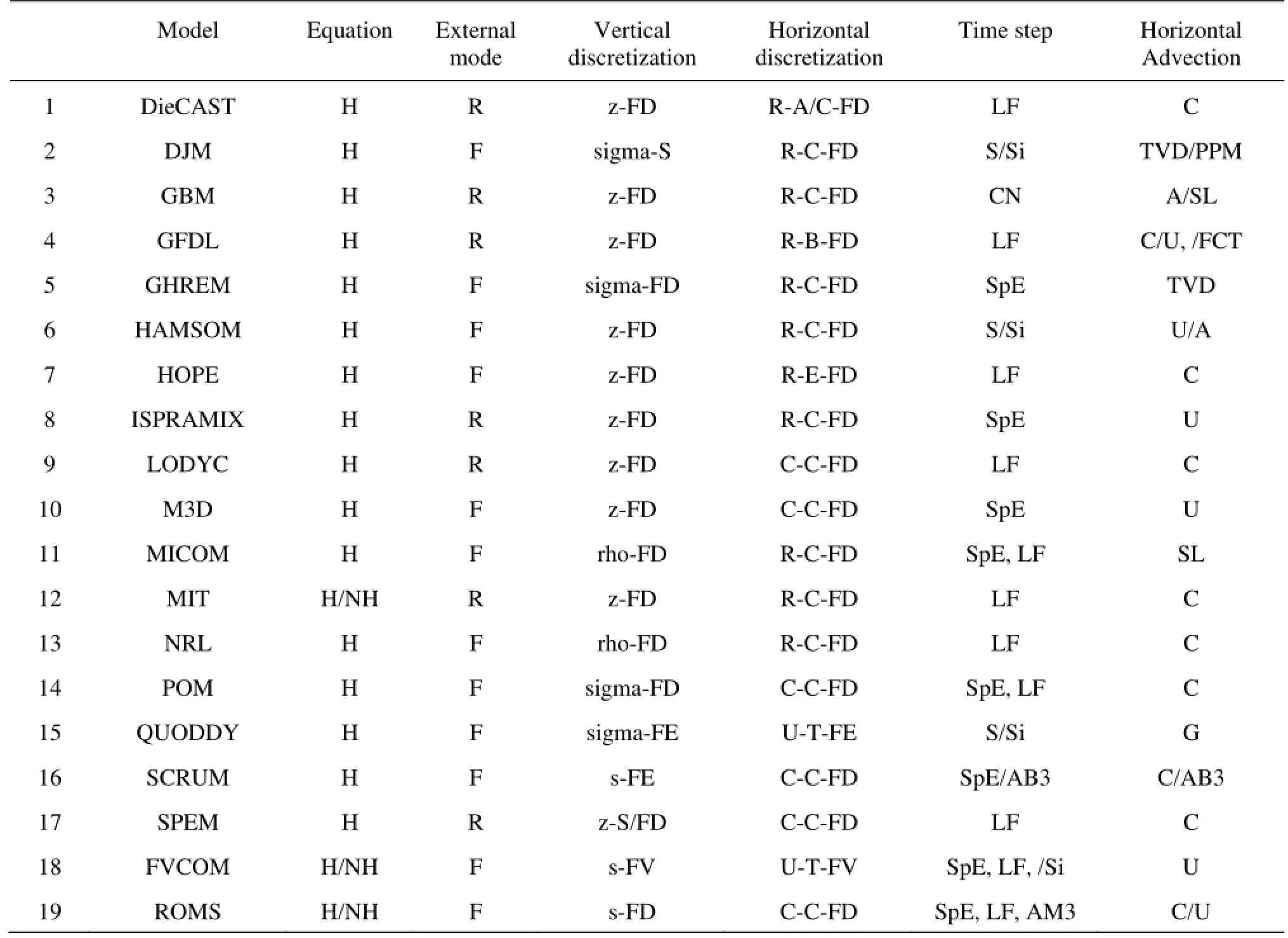
Table 1 Review of the historical and current three-dimensional ocean circulation models and their features
By contrast, in a two-level time difference scheme, the information of only one previous time level is used instead of two time levels like the three-level scheme. Thus the two-level scheme is immune to the computational mode which is inherent in the threelevel scheme. One way is to use the multistage technique to achieve a higher-order accuracy in the twolevel scheme by estimating the prognostic variable at several intermediate instants, such as the Runge-Kutta algorithms. For example, an attempt was made to re-place the leapfrog scheme with a second-order Runge-Kutta scheme in an atmospheric general circulation model, NCAR CAM3.0 (Community Atmosphere Model 3.0), and an improvement in the long-term climate simulation was reported[7]. However, secondorder Runge-Kutta schemes require evaluating righthand-side functions twice per time step and would also lead to slowly growing instabilities. The fourthorder Runge-Kutta schemes are highly accurate but require four function evaluations per time step. Another practical alternative is the Eulerian forward-backward difference scheme (FB for short afterwards), which is effectively centered in time and of second-order accuracy (Shchepetkin and McWilliams, 2005, private communication with Durran). It was widely used in many models for the barotropic mode. Another advantage of the FB scheme over the leapfrog is its better stability. For a staggered grid, the critical Courant number of the FB method is 1 while it is 0.5 for the leapfrog scheme[5], which means that the FB scheme is “clearly economical with a stable time step twice as large as the leapfrog scheme”[8].
In this paper, we apply the FB scheme in the baroclinic circulation model and build a finite-differenced, mode-splitting, and free-surface three-dimensional ocean circulation model with the FB scheme as the time-stepping algorithm in both internal and external modes (also called the baroclinic and barotropic modes, respectively). This model is named the“MASNUM” ocean circulation model after the name of our laboratory (The Key Laboratory of the Marine Sciences and Numerical Modeling, State Oceanic Administration of China). The MASNUM ocean circulation model is based on the Reynolds-averaged primitive equations of the oceanic motions under the terrain-following coordinates. The Boussinesq approximation and the primitive-equation-model approximations (with the hydrostatic approximation included) are used to establish the physical ground of the numerical model. Some unresolvable sub-grid motions in the circulation model, such as the isotropic turbulence, the surface gravity waves, and the mesoscale eddies, are treated as the disturbances of different kinds in the motion decomposition. Their effects on the large-scale circulation motions, i.e., the second-order-moment terms are explicitly expressed through Reynolds-averaging procedures.
For testing the performances of the MASNUM circulation model, the tides of the east China Seas, a barotropic phenomenon, and the Yellow-Sea cold water mass, a baroclinic phenomenon, are simulated. To further verify the reliability of the MASNUM circulation model, a thorough comparison of the time series of some prognostic variables between the MASNUM and POM circulation models is made in the simulation of the northwest Pacific under the same model setup.
1. Model equations
The RANS equations for the large-scale circulation are normally used for the model’s numerical integration,
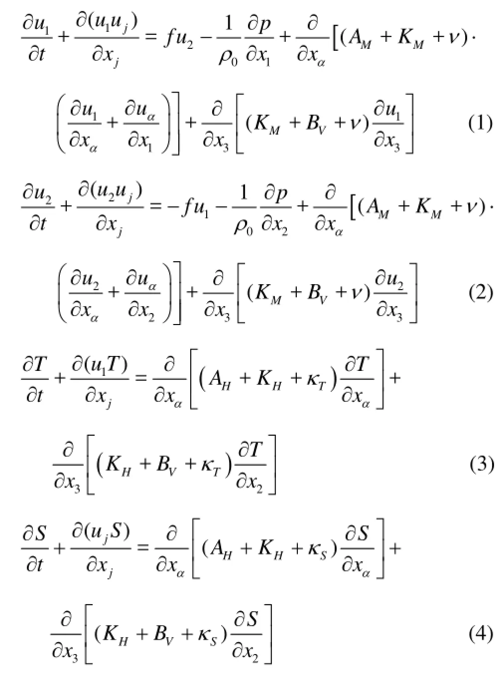
The turbulence is modeled by the Mellor-Yamada’sq2-lclosure model. It is a two-equation turbulence model first applied in the POM circulation model.
The governing Eqs.(1)-(4) are derived in the conventional Cartesian coordinate system withzcoordinate. We adopt the terrain-following coordinate system (the sigma coordinate system) in our model, where, the vertical kinetic boundary conditions can be greatly simplified and be made linear and homogeneous. The staggered Arakawa-C grid is adopted as the horizontal mesh grid in our model. The three-dimensional setup of the meshes is vertically terrain-following, and horizontally orthogonal.
2. Forward-backward scheme and its numerical features
In most of the three-dimensional circulation models, three-level explicit schemes are used for temporal differencing, among which the leapfrog scheme is the most popular. The two-level explicit schemes are absent in the three-dimensional circulation models listed in Table 1. As mentioned in the introduction, the two-level schemes are naturally free of the computational mode inherent in the three-level schemes. The Runge-Kutta methods are typical two-level schemes with good orders of accuracy. However, the Runge-Kutta schemes are a multi-stage method, implying that the right-hand-side terms of the prognostic equations have to be evaluated more than once within one integration time step, thus less efficient than the singlestage method.
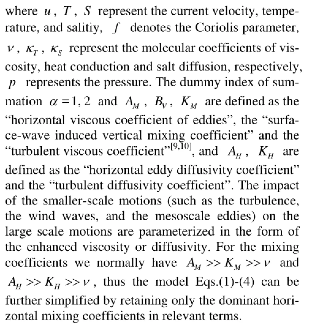
Table 2 Comparison of the numerical characteristics of FB, leapfrog and Asselin-filtered leapfrog schemes
Sun adopted the FB method in the finite volume model to simulate the dam break by solving the shallow-water equations[8,11]. This method is also commonly used in the barotropic mode of a three-dimensional ocean circulation model[12]. But the application of the FB scheme as the only time-stepping algorithm in three-dimensional ocean circulation models has not been attempted as far as we know.
The numerical characteristics between the FB scheme and the leapfrog schemes (the original one and the Asselin-filtered leapfrog) are compared as shown in Table 2. The filter coefficient 0.1 is used in assessing the order of accuracy of the Asselin-filtered leapfrog scheme for a clearer comparison. The weakness of the leapfrog scheme is its undamped computational mode, which is slowly amplified during the simulations of nonlinear wave propagation problems, which would generate an instability known as “time splitting”[5]. The FB differencing involves only two time levels thereby the introduction of computational modes is avoided.
3. Validation of the MASNUM circulation model
The same as a mode-splitting, terrain-following coordinated ocean circulation model, the POM model is used as a reference to verify the applicability of the two-time-level MASNUM circulation model in this paper. As a result, we use the same algorithms as in the POM model in this version of our model. These algorithms include the Equation of State for the seawater, the Mellor-Yamada level-2.5 turbulence closure model of the two-level scheme version, and the straightforward discretization algorithm of the pressure gradient force[9]. The numerical framework of the time stepping is totally different due to the adoption of a two-time-level scheme.
Three experiments are carried out to examine the performance of the MASNUM circulation model. The barotropic and baroclinic responses of the model are investigated by a tidal simulation experiment with a strong baroclinic phenomenon in the summer of the Yellow Sea. Besides, a thorough comparison of the modeled quantities between the POM model and MASNUM model are made.
3.1Barotropic response of the model: Tidal simula
tion experiment
As the first step to inspect the performance of the MASNUM circulation model, a tidal simulation experiment is conducted to compute the tides in the China Seas. The experiment includes a two-dimensional run and a three-dimensional run. The two-dimensional run disables all the thermodynamic mechanisms, with only the external mode activated in the model simulation. This model run is equivalent to a shallow-water equation model. By contrast, both internal and external modes in the circulation model are activated in the three-dimensional run. The effects of stratification on the tidal wave propagation can be revealed by comparing the results of the two model runs.
The correct response to the barotropic forcing is one of the most basic simulation capabilities for a three-dimensional circulation model. The tide is a typical barotropic phenomenon. The periodic surfacefluctuations and tidal currents are attributed to the propagation of tidal waves, as shallow-water gravity waves. Thus the tidal waves can be used for inspecting the response of the MASNUM circulation model to the barotropic forcing. It is mainly the external mode of the circulation model tested by the tidal simulation experiment because of the fast propagating speed of the tidal waves.
In our tidal simulation experiment, the numerical area involves the Bohai Sea, the Yellow Sea and the East China Sea, i.e., the marginal seas within 24oN-41oN and 117oE-131oE excluding the Japan Sea and the southeast to the Okinawa trough. The horizontal spatial resolution is 1/6oin both latitude and longitude, and the vertical dimension is discretized into 9 sigma layers. The Etopo5 data provide the topography for the model. The initial temperature and salinity fields required in the three-dimensional run are prescribed by the annual mean Levitus climatology.
As a test of barotropic response, the experiment includes the tidal wave at the lateral open boundary as the only forcing mechanism for the model, and excludes the surface fluxes (such as momentum, heat, and freshwater) in the model simulation. Only a tidal constituent M2is considered in the tidal forcing because the M2component is quite dominant in the area of study and it is simpler and more accurate to perform the harmonic analysis if with only one tidal component. The surface elevationηis prescribed at the open boundary as,
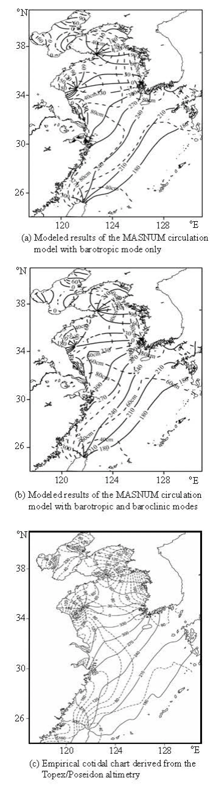
Fig.1 Comparison of the cotidal charts of M2component in the marginal seas of China. The solid and dashed lines represent the phase lag and the tidal amplitude of the component M2
Therefore, this experiment has preliminarily validated the performance of the MASNUM circulation model to the barotropic forcing. The inclusion of the density stratification in the tidal simulation could improve the accuracy in the phase lag to some extent. The reduction in the amplitude compared with the empirical cotidal chart derived from the satellite altimetry may result from the default setup of the bottom friction.
3.2Baroclinic response of the model: simulation of
Yellow Sea Cold Water Mass
The Yellow Sea is a marginal sea of the northwest Pacific with Korean Peninsula to the east and the China mainland to the west. To the south it is open to the East China Sea and the estuary of Yangtze River, the third longest river in the world.
The water of the Yellow Sea shows remarkable seasonal variations due to the shallow environment (average depth of 44 m) and the monsoon. However, the water in the central trough of the Yellow Sea displays less seasonal variability. The water at the central trough in spring is a remnant of the cold, vertically well-mixed water in the previous winter and remains hardly affected by the increased surface heating in spring and summer as a result of its depth. A strong thermocline thus develops above the cold water mass and suppresses the downward heat transfer. On the other hand, the tidal mixing effect is quite efficient to break down the seasonal thermocline in summer in the shallow waters approaching the shore. Thus the temperature gradients around the cold water become sharper and form remarkable fronts through spring and summer, which creates the dome-like temperature patterns on the trough. The stable cold water on the trough does not collapse until winter and can maintain as long as half a year. Because it is more noticeable in the temperature field, this cold water is called the Yellow Sea Cold Water Mass (YSCWM for short afterwards) or the Yellow Sea Bottom Cold Water[15]. It is widely accepted that this typical baroclinic phenomenon is attributed to the joint effects of the tidal mixing, the bottom topography and the surface heat flux.
To verify the performance of the MASNUM circulation model in simulating the baroclinic phenomenon, we set up a numerical experiment to simulate the YSCWM and compare the model results with the observations.
The MASNUM circulation model spins up for 3 years from the quiescent state to yield a relatively stable circulation background. Some optional mechanisms are excluded in the spin-up process, such as the surface-wave mixing, the Yangtze River diluting water and the tidal-current forcing. After three years’integration, the model continues to run for another year with all these optional mechanisms included.
The effect of the tidal currents is introduced by prescribing the vertically-integrated current at the open boundary. The time-dependent tidal currents are determined from the tidal levels if the tidal waves at the boundary can be regarded as progressive waves,


The simulation result of the fourth year with all aforementioned optional mechanisms activated in the MASNUM circulation model is used for comparison with the observations. The First Institute of Oceanography of China and the Korean Ocean Research and Development Institute jointly carried out six extensive field surveys on the YSCWM during the period of 1996–1998. The range of each field survey covers extensively the whole southern part of the Yellow Sea from west to east. Six major zonal transects marked A-F from 37oN to 32oN were obtained in each cruise. CTD data were obtained by using SeaBird 9/11 and SeaBird 25, equipped with dual temperature and electrical conductivity sensors.
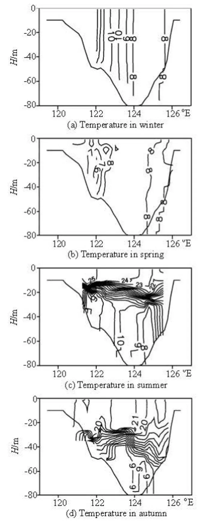
Fig.2 Transect contours of the observed temperature along the 35oN transect, reproduced from Xia et al.[13]
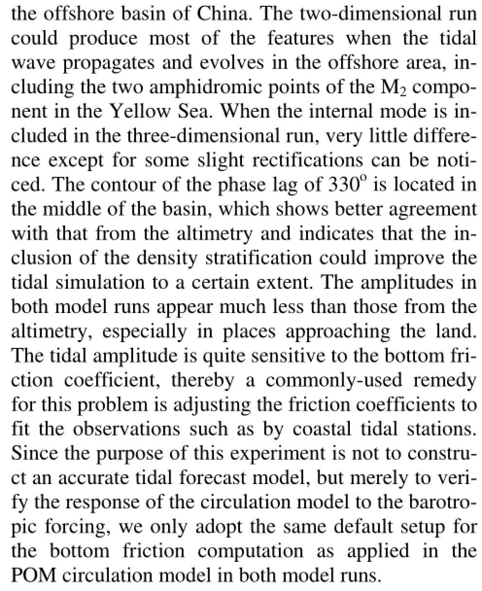
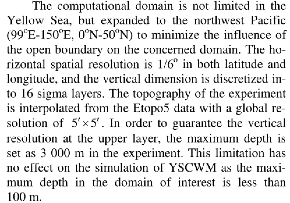
Many researches were conducted based on the data collected in the China-Korea cooperation field survey in the Yellow Sea. In this paper we adopt the transect-distribution of the temperature along four transects plotted by Xia et al.[13]for the model verification, including the transect distributions of the temperature along a longitudinal transect along 124oE and a zonal transect along 35oN for four selected cruises which were conducted within typical months of four seasons: winter (February, 1997), spring (April, 1996), summer (July, 1997) and autumn (October, 1996).

Fig.3 Transect contours of the modeled temperature by the MASNUM circulation model along the 35oN transect
The transect contours of the temperature along the section 35°N in four seasons are reproduced in Fig.2[13], while the contours of the modeled temperature by the MASNUM circulation model in the same months are shown in Fig.3. The modeled temperature shows a notable dome-like pattern of the bottom cold water in summer and autumn, and the uniform distribution throughout the vertical water column in winter. Other features of YSCWM such as “the kernel temperature of the cold water mass is below 10oC”, “the cold water mass only appears in the summer halfyear”, “the cold water mass peaks within July and August” are also discovered in the simulation results. It is worth emphasizing that the surface forcing applied in the experiment is the climatological data instead of the real-time observations, which may account for part of the differences in details between the model simulation and the field investigation.
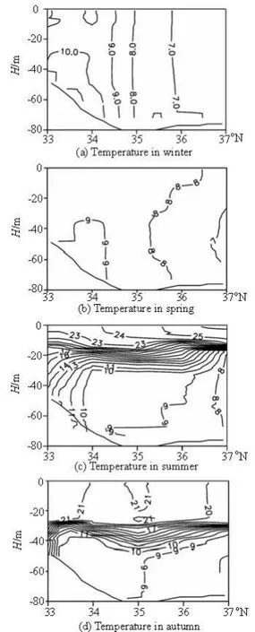
Fig.4 Transect contours of the observed temperature along the124oE transect reproduced from Xia et al.[13]

Fig.5 Transect contours of the modeled temperature by the MASNUM circulation model along the 124oE transect
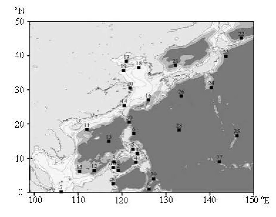
Fig.6 Topography of the northwest Pacific and the distribution of the selected 30 computational points for time-history comparison. Locations of these points are marked by black squares with the index number (pid) upon each
The contours of the observed temperature along the transect 124oE in four seasons are also reproduced in Fig.4. The corresponding simulation results of the MASNUM circulation model are shown in Fig.5. The well mixing pattern in winter and the remarkable front around the cold water mass in summer and autumn are also well simulated by the model.
It can be concluded that the model could simulate the main features of the seasonal evolution of the YSCWM and produce results that agree well with the observations in different seasons. Thedifferencesbetween the model simulation and the field investigation are partly due to the climatological forcing data.
3.3Comparison between the POM and MASNUM cir culation models
The performance of the MASNUM circulation model is tested by barotropic and baroclinic experiments in the previous sections. A few specific prognostic variables are compared with the observations at some particular time of the year. To further validate the reliability of the MASNUM circulation model, a through comparison with the well-developed POM circulation model is made for a regional simulation.
The most important difference between the POM and MASNUM models is the time-stepping framework. In the POM model, a three-level scheme is applied, which requires the information from the previous two time levels in stepping forward to the next; while in the MASNUM model, a two-level scheme is used, which involves data of only one earlier time level in the time integration. This difference is fundamental for the numerical models because there is only half information available in the term evaluation for the twolevel schemes as compared with the three-level schemes. Therefore, the algorithm for every term in the prognostic equations differs significantly between the two-level and three-level schemes. However, a nondissipative computational mode is inherent in the leapfrog time-difference scheme, as a typical three-level scheme adopted in the POM model. The Asselin filtering is introduced to remove the computational mode and control the nonlinear instability as well. But for the forward-backward (FB) scheme, with an Eulerian two-level scheme adopted in the MASNUM circulation model, it is not necessary to remove the computational mode. Only a simple smoothing method is employed to control the nonlinear instability.
Despite of the problem in the numerical scheme, the POM model can still provide reliable simulation results for a wide-range of hydrodynamic problems. The comparison with a mature model is an effective way or even an obligatory procedure to test the simulation performances for a new model. In order to minimize the difference other than that due to the numerical schemes, in the MASNUM model, the same algorithms of the internal pressure gradient force and the equation of state are used as those in the POM model. The evaluation of the turbulence mixing coefficients in the MASNUM model also follows the Mellor-Yamada level-2.5 turbulence closure model as incorporated in the POM model only that the original algorithm is transformed to the FB scheme version.
We adopt the spin-up process in simulating the northwest Pacific mentioned in the previous section for the model comparison. Both the POM model and the MASNUM model are set up to run for 3 years from the quiescent state. The surface forcings include the wind stress and the heat fluxes from the climatological data. The circulation currents prescribed at the lateral open boundary are interpolated from those of a global model run with coarse resolutions[13]. Details are in the previous section for setups of the model simulation.
To make the comparison as convincing as possible, the complete time history of four prognostic variables is compared in 30 computational points selected in some arbitrary way. The time history in the comparison ranges from the beginning of the integration till the end of the third year. The four prognostic variables selected for the comparison are the surface elevation in the external modeη, the meridional component of the vertically-averaged current velocity in the external modeav, the zonal component of the three-dimensional current velocity in the internal modefu, and the (potential) temperatureT. These four variables are selected deliberately out of the seven prognostic variables. They can be regarded as the representatives of two internal and two external variables, or two two-dimensional and two three-dimensional variables, or two scalars and two vector components, or one thermodynamic and three kinetic parameters. The locations of the selected computational points for the comparison are marked in Fig.6. The points are selected around some typical areas, and those with complicated topographic conditions are not avoided. These points scatter all over the computational domain and are representative of the whole area.
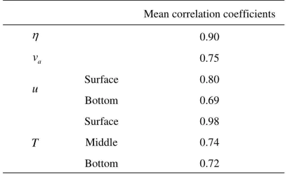
Table 3 Statistics of the mean correlation coefficient of the time histories of both models
The correlation coefficients of the time histories from both circulation models for the selected four prognostic variables are obtained at the selected 30 computational points as shown in Table 3. The correlation coefficients for quantities with vertical structures (fuandT) are evaluated at some certain layers (such as the surface, the bottom, or the middle layer) at each point. It is found that over 50% of the correlation coefficients in the table exceed 0.9, which implies that the simulation results of the two models agree quite wellwith each other. However, there are also some negative correlations in the table. To clarify the bad correlations, the complete time histories of 1 080 d for the variablesη,av,fuandTfrom the MASNUM model are compared with those from the POM model at four representative points as shown in Fig.7-Fig.9.
The time history of pid-9 (Fig.7) represents cases with bad correlations. We find that the small even negative coefficients of correlation usually occur in the time histories whose ranges of values are so limited that very minor fluctuations will affect the patterns to a notable extent and then play an important role in the correlations between the two models. Take the negative correlation in the middle-level temperature at pid-9 as an example, the fluctuation range of the temperature is within only 0.5oC during most time of the integration. Such points still include pid-25 and pid-29.

Fig.7 The complete time histories of three years for the quantities at pid-9. The grey lines represent the POM model, and the black lines represent the MASNUM model
The time history of pid-16 (Fig.8) represents the trough areas with sharp slopes in topography. The time history in Fig.8 shows surprisingly a good consistency between the two models. Such points include pid-24. But the correlations of some trough points such as pid-25 and pid-27 are not as good, which may be explained by the same reason as for the point of pid-9 in the last paragraph.
The time history of pid-20 (Fig.9) represents the coastal points, for example, pid-17, pid-18 and pid-19. The correlations between the two models at those points are also quite goo d.
Ingeneral,thetimehistoriesinvolvedinthecomparison between the two models show a quite good consistency in both amplitude and phase at most of the computational points. This comparison further shows the reliability and applicability of the two-level time-differencing, three-dimensional circulation model.
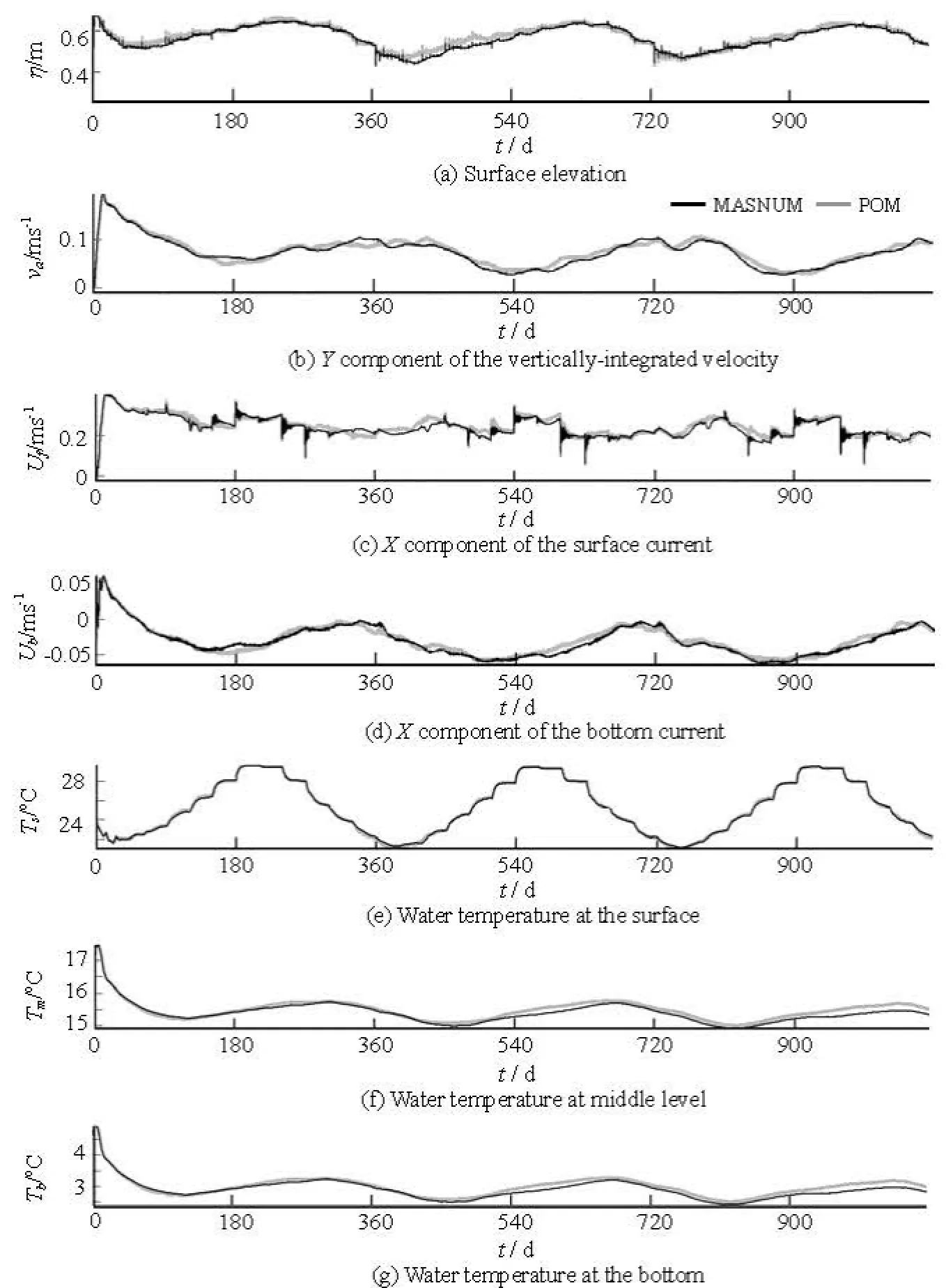
Fig.8 The same as Fig.7, but for pid-16
4. Conclusions
The numerical characteristics of the applicable ocean circulation models are reviewed, where no twotime-level explicit schemes are used in time stepping. The three-level leapfrog scheme is most preferred and frequently adopted in a newly-built finite-differenced circulation model (the MASNUM circulation model). The leapfrog scheme is indeed preferable to many other schemes in the numerical stability, the order of accuracy and the computational economy. But the non-damping computational mode inherent in the original leapfrog scheme will develop in nonlinear problems and eventually dominate the solution. Many strategies were employed to control the leapfrog computational mode, but the order of accuracy or the numerical efficiency would be degraded. In this paper, the three-time-level methods are abandoned and the FB method, a simple two-time-level scheme, is adopted to construct a baroclinic ocean circulation model. The FB method is also of the second order of accuracy and requires only once of the function evaluation as the original leapfrog scheme, but it is free of the computational mode for it only involves two time levels. Furthermore, the FB scheme is more economical witha stable time step twice as large as the leapfrog scheme under staggered grids.
With the Reynolds-averaged governing equations, the motions unresolvable for the circulation model are treated as the fluctuations to the circulations. With the Reynolds decomposition method, the unresolved motions with different scales and mechanisms are separated and explicitly expressed in the form of the secondorder moments, which indicate the influences of the unresolved disturbances to the large-scale motions. In this paper, three disturbances are considered: the mesoscale eddies, the surface gravity waves, and the isotropic turbulence. Various parameterization algorithms are introduced to calculate the second-order moments of the Reynolds averaging.
Three experiments are conducted to examine the performance of the MASNUM circulation model. The first experiment tests the barotropic responses of the model by a tidal simulation in the marginal seas of China. The second experiment simulates a strong baroclinic phenomenon in the summer of the Yellow Sea. The third is a thorough comparison of the modeled quantities between the POM model and the MASNUM model.
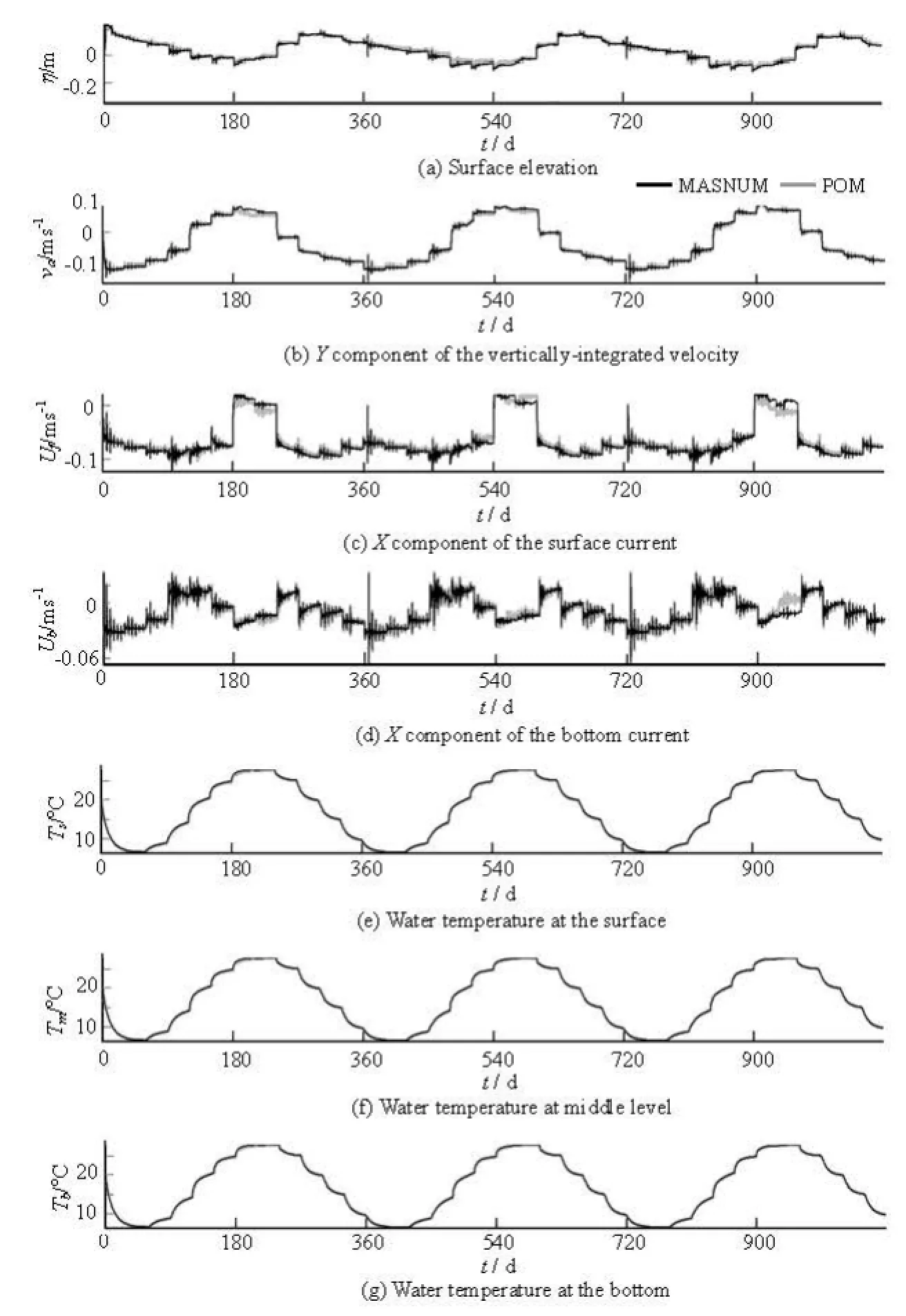
Fig.9 The same as Fig.7, but for pid-20
In the first experiment, both the amplitude and the phase lag of M2component numerically simulated by the MASNUM circulation model agree well with those from the Topex/Poseidon altimetry in the offshore basin of China. Besides, the inclusion of the density stratification in the tidal simulation may improve the accuracy in the phase lag to some extent.
In the second experiment, the MASNUM circula-tion model is set up to simulate the area of northwest Pacific. The strong baroclinic features of the Yellow Sea Cold Water Mass and its seasonal evolution are well simulated by the MASNUM circulation model. The differences in details between the model simulation and the field observation are partly due to the climatological forcing data instead of the real-time observations used in the model.
The third experiment is performed to validate the reliability in a more thorough way. The POM circulation model also with the terrain-following coordinate is used as a reference model to test the results by the MASNUM circulation model. The three-year time histories of four prognostic variables in 30 representative computational points in the northwest Pacific area obtained by the two models are compared. The correlations are quite good for most areas, except for the quantities whose ranges of values are so limited that very minor fluctuations would affect the patterns to a notable extent and then played an important role in the correlations. In overall, the comparisons of the time histories show a quite good consistency in both amplitude and phase at most of the computational points. This comparison further shows the reliability and applicability of the two-level time-differenced three-dimensional circulation model. Besides, due to the simpler time stepping algorithm, the MASNUM circulation model could gain another 8% decrease in the execution time than the efficient POM model under the same computational environment.
By these three numerical experiments, we may conclude that the two-level scheme is feasible for the baroclinic three-dimensional ocean circulation models. The forward-backward method is simple and superior to many other schemes. It is effectively centered in time with the second order of accuracy, it is efficient in the numerical integration with only once of the function evaluation required per time step, and it is stable with the maximum allowed Courant number not reduced for the staggered grids. The newly-built MANSUM circulation model exclusively employing the FB scheme in both barotropic and baroclinic modes are preliminarily shown to be reliable and applicable in simulating the oceans. More tests and experiments will be performed to further verify this twotime-level model.
Acknowledgement
The authors thank the anonymous reviewers for their careful reviews and constructive comments in improving the original manuscript, and the editors who kindly polished this article with great effort.
[1] KANTHA L. H., CLAYSON C. A. Numerical models of oceans and oceanic processes[M]. Waltham, Massachusetts, USA: Academic Press, 2000.
[2] CHEN C., LIU H. and BEARDSLEY R. C. An unstructured grid, finite-volume, three-dimensional, primitive equations ocean model: Application to coastal ocean and estuaries[J]. Journal Atmospheric and Oceanic Technology, 2003, 20(1): 159-186.
[3] CHEN C., BEARDSLEY R. C. and COWLES G. An unstructured grid, finite-volume coastal ocean model (FVCOM) system[J]. Oceanography, 2006, 19(1): 78-89.
[4] HAIDVOGEL D. B., ARANGO H. and BUDGELL W. P. et al. Ocean forecasting in terrain-following coordinates: Formulation and skill assessment of the regional ocean modeling system[J]. Journal of Computational Physics, 2008, 227(7): 3595-3624.
[5] DURRAN D. R. Numerical methods for wave equations in geophysical fluid dynamics[M]. New York, USA: Springer, 1999.
[6] MARSALEIX P., AUCLAIR F. and DUHAUT T. et al. Alternatives to the Robert-Asselin filter[J]. Ocean Modelling, 2012, 41: 53-66.
[7] ZHAO B., ZHONG Q. An alternative method to leapfrog time differencing and its applications in an atmospheric general circulation model[J]. Climatic and Environmental Research, 2009, 14(1): 21-30.
[8] SUN W.-Y. Instability in leapfrog and forward-backward schemes[J]. Monthly Weather Review, 2010, 138(5): 1497-1501.
[9] MELLOR G. L. Users guide for a three-dimensional, primitive equation, numerical ocean model[M]. Princeton, New Jersey, USA: Atmospheric and Oceanic Sciences Program, Princeton University, 2003.
[10] QIAO F., YUAN Y. and YANG Y. et al. Wave-induced mixing in the upper ocean: Distribution and application in a global ocean circulation model[J]. Geophysical Research Letter, 2004, 31(11): L11303.
[11] SUN W.-Y. Instability in leapfrog and forward-backward schemes Part II: Numerical simulations of dam break[J]. Computers and Fluids, 2011, 45(1): 70-76.
[12] SHCHEPETKIN A. F., MCWILLIAMS J. C. The regional ocean modeling system: A split-explicit, freesurface, topography following coordinates ocean model[J]. Ocean Modelling, 2005, 9(4): 347-404.
[13] XIA C., QIAO F. and YANG Y. et al. Three-dimensional structure of the summertime circulation in the Yellow Sea from a wave-tide-circulation coupled model[J]. Journal of Geophysical Research, 2006, 111(C11): C11S03.
[14] FANG G., WANG Y. and WEI Z. et al. Empirical cotidal charts of the Bohai, Yellow, and East China Seas from 10 years of TOPEX/Poseidon altimetry[J]. Journal of Geophysical Research, 2004, 109(C11): C11006.
[15] PARK S., CHU P. C. and LEE J.-H. Interannual-to-interdecadal variability of the Yellow Sea Cold Water Mass in 1967-2008: Characteristics and seasonal forcings[J]. Journal of Marine System, 2011, 87(3-4): 177-193.
10.1016/S1001-6058(14)60005-6
* Project supported by the National Science Foundation of China (Grant No. 40906017, 41376038), the National High Technology Research and Development Program of China (863 Program, Grant No. 2013AA09A506).
Biography: HAN Lei (1981-), Male, Ph. D. Senior Engineer
杂志排行

水动力学研究与进展 B辑的其它文章
- Deepwater gas kick simulation with consideration of the gas hydrate phase transition*
- Detrended analysis of Reynolds stress in a decaying turbulent flow in a wind tunnel with active grids*
- Estimation of discharge and its distribution in compound channels*
- Influences of soil hydraulic and mechanical parameters on land subsidence and ground fissures caused by groundwater exploitation*
- A hybrid DEM/CFD approach for solid-liquid flows*
- Scale analysis of turbulent channel flow with varying pressure gradient*