Balance control of a 12-DOF mobile manipulator based on two-wheel inverted pendulum robot

Gang Wang, Seunghwan Choi, Jangmyung Lee

(Dept.of Electrical Engineering, Pusan University, Busan 609-735, Korea)

Balance control of a 12-DOF mobile manipulator based on two-wheel inverted pendulum robot

Gang Wang, Seunghwan Choi, Jangmyung Lee

(Dept.of Electrical Engineering, Pusan University, Busan 609-735, Korea)

Humanoid mobile manipulator which is based on two-wheel inverted pendulum robot has been studied. Balance control is a key problem for this kind of centroid-variable robot. Due to the principle of two wheel inverted pendulum, a timely angle compensation is necessary to make the system keep balance when the centroid changes. In this paper, a method based on coordinate transformation is introduced to get the compensatory angle and a 12-DOF mobile manipulator is also used to check the method. Simulation and experimental results show the effectiveness of the method.

angle compensation; inverted pendulum; variable centroid; humanoid

Manipulators have been widely used in factory nowadays. Most of them are installed on a fixed place. Mobile manipulators have attracted more attention in recent years because they can work under uncertain surroundings. Most of this kind of robot have been developed based on a stable platform. In Ref.[1], they introduced a mobile manipulator with a LABNATE platform. A cooperation method between several mobile manipulators was introduced in Ref.[2], and these robots were all with a stable platform. Coordinated task execution of a human and a mobile manipulator was presented in Ref.[3]. After Segway appeared in 2002, more attention was attracted by this kind of platform[4]. Mobile manipulator developed in Keio University was a one-arm manipulator which is based on Segway platform[5]. EMIEW was a two-wheel humanoid service robot with a relatively stable centroid[6]. When a manipulator based on two-wheel inverted pendulum has an obviously time-variant centroid, balance control comes to be a big problem. To do some research on this problem, a 12-DOF mobile manipulator is developed in this paper.

1 Mathematical model of centroid

Establishing the model of centroid is helpful to get the compensatory angle of the body. By given position of centroid, statement control of the robot is available.

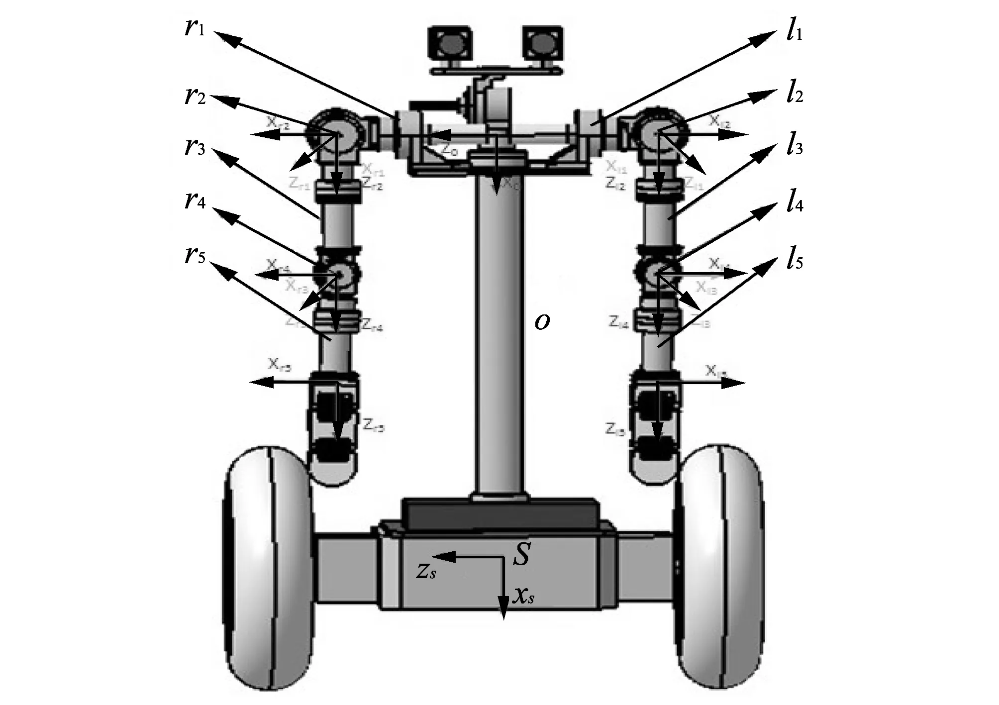
Fig.1 Model of the robot with 12 coordinate systems

As shown in Fig.1, the robot introduced in this paper mainly includes two parts: the upper one is a 10-DOF (except camera) dual arm manipulator, and the chassis is a two-wheel inverted pendulum robot. By connecting the manipulator to chassis with a passive joint, the robot gets 12 active joints and 1 passive joint in this robot. Making Cartesian coordinate systems as shown in Fig.1, then coordinate transformation by D-H method can be got. D-H parameters of the robot are shown in Table 1 and Table 2.

Table 1 D-H parameters for left arm

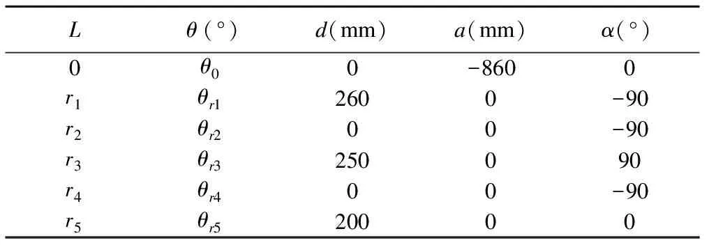
Table 2 D-H parameters for right arm

So, transformation matrix for the first line is

where c0means cosθ0; s0means sinθ0. In this way,0Hl1,l1Hl2,l2Hl3,l3Hl4,l4Hl5,0Hr1,r1Hr2,r2Hr3,r3Hr4andr4Hr5can be got.

Transformation matrices from each coordinate system to S coordinate are shown as

The position of each centroid in XsYsZscoordinate system is expressed by

where i∈(0,l1,l2,l3,l4,l5,r1,r2,r3,r4,r5,s); (sxi,syi,szi) means the i-th centroid coordinate expressed in XsYsZssystem. And then the centroid position of the whole body will be

where (sxc,syc,szc) denotes the coordinate of centroid expressed in XsYsZssystem. So it is possible to get the compensatory angle in XsOYsplane, namely,

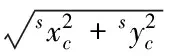
And the length from centroid to zero which belongs to XsOYsplane should be

(15)

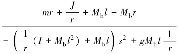
2 Dynamic model

Dynamic model can help analyze and control the system. A dynamic model of the robot introduced is shown in Fig.2. In this model, the robot is divided into two parts. In Fig.2(a), force analysis of wheel is proposed and Fig.2(b), the main body of the robot is seen as a virtual body which includes the centroid and a virtual link.

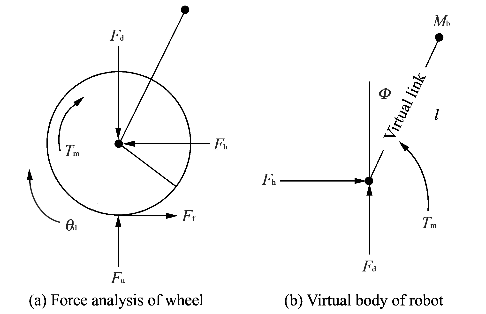
Fig.2 Dynamic model of the robot

In Fig.2, Fdis the vertical force between wheel and body, Fhis the horizontal force between them, Tmis the torque produced by motors, r is the radius of wheel, θwis the rotation angle of wheel, Mbis the mass of robot body, Φ is the tilt angle of centroid- Fuand Ffrepresent the force given by ground vertically and friction, respectively.

Movement of wheel can be divided into horizontal movement and rotation movement. For horizontal!movement, its kinematic equation is

where v and m denote velocity and mass of wheel, respectively. For rotation movement, the kinematic equation is wirtten as

where J and ω represent moment of inertia and angle velocity of wheel, respectively.

Taking Eq.(17) into Eq.(16), then Eq.(18) can be got as

Assume that there is no sliding happened between wheel and ground, and then Eq.(18) can be rewritten as

where v=ωr.

Robot body is seen as a centroid and a virtual link. Movement of body also can be divided into two parts as wheel. For vertical direction, kinematic equation is

where lvis vertical position of centroid.

For horizontal direction, kinematic equation is

where lhis horizontal position of centroid.

From Fig.2, lvand lhcan be derived as

where p0is horizontal position of wheel axis.

where Φ=θ+θtiltand θtiltis the tilt angle of platform.

Kinematic equation of rotation of body is

where I is moment inertia to axis produced by robot body.

Then taking Eqs.(24) and (25) into Eqs.(20) and (21), Fdand Fhcan be got, taking Fdand Fhinto Eq.(26), then

where l is just seen as a constant.

Taking v=ωr into Eq.(27), and then taking Tminto Eq.(19), when Φ just changes from -5° to 5°, linearization is made around 0. Taking sinΦ=Φ and cosΦ=1 into consideration, dynamic equation of the robot is

(29)

Eq.(29) can be rewritten as

where

(33)

3 Simulation of centroid

Simulation about centroid can check the accuracy of equations got above and get influence of each joint to centroid. The simulation results of joint and influence are not included in this paper. The first and fourth joints of each arm have more obvious influence to centroid, these 4 joint will be taken out to finish the experiment. Fig.3 shows partial simulation results.

Mathematic simulation shows that when the first joint moves forward, the centroid will also move forward, and so do the other joints, respectively. In Fig.4(a), it shows the relation between θl1, θr1and compensatory angle, Fig.4 (b) shows the relation between θl1, θl4and compensatory angle. These results are used to compare with the experiment data.

Simulation results are used to check the relation between position of centroid and angles of each joint. Follow these results, compensatory angle for whole body can be checked.

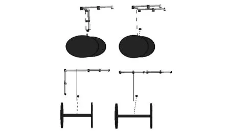
Fig.3 Simulation results of centroid. The dot is centroid of whole body, first two pictures are about side face, and another two are about front side

Fig.4 Mathematics simulation results

4 Communication structure, controller and experimental results

4.1 Communication structure of the whole body

In this system, there are ten AVR for manipulator and one ARM for mobile platform.In order to calculate the position of centroid,another singlechip is necessary. So in this system, the 11th AVR is used as a centroid calculator and data collector. Basic method of communication is call and answer. The calculator can get 10 sets of data from each AVR in a second. This will make sure that the calculator can get the position of centroid in time.

As shown in Fig.5, L1to L5and R1to R5represent the controller of each joint and C means the calculator for position of centroid, which is connected to ARM by an UART port. RS232 is used to connect C with other AVR because only UART communication can not make it well.

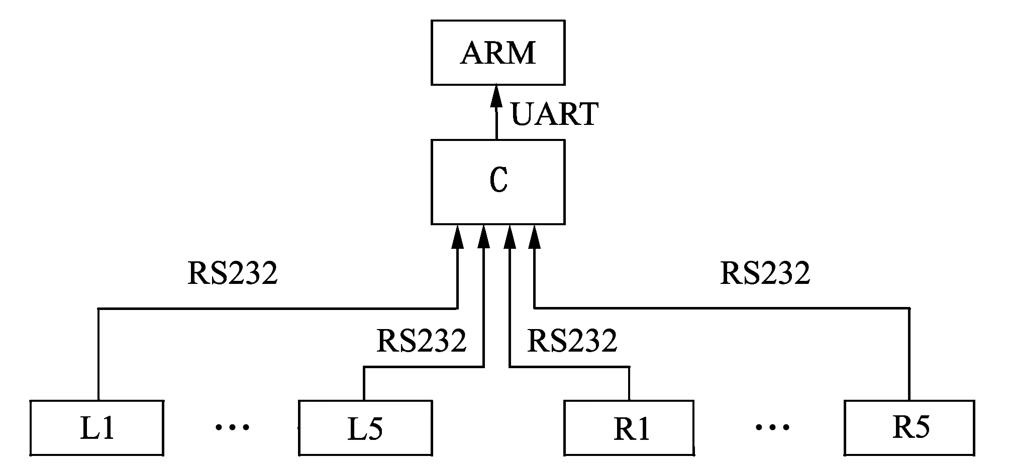
Fig.5 Communication structure of the system

4.2 Controller illustration

Normally, PID control is widely used in this kind of inverted pendulum robot. But we can not get the position of centroid so exactly, the PD control is used in this paper, as shown in Fig.6.

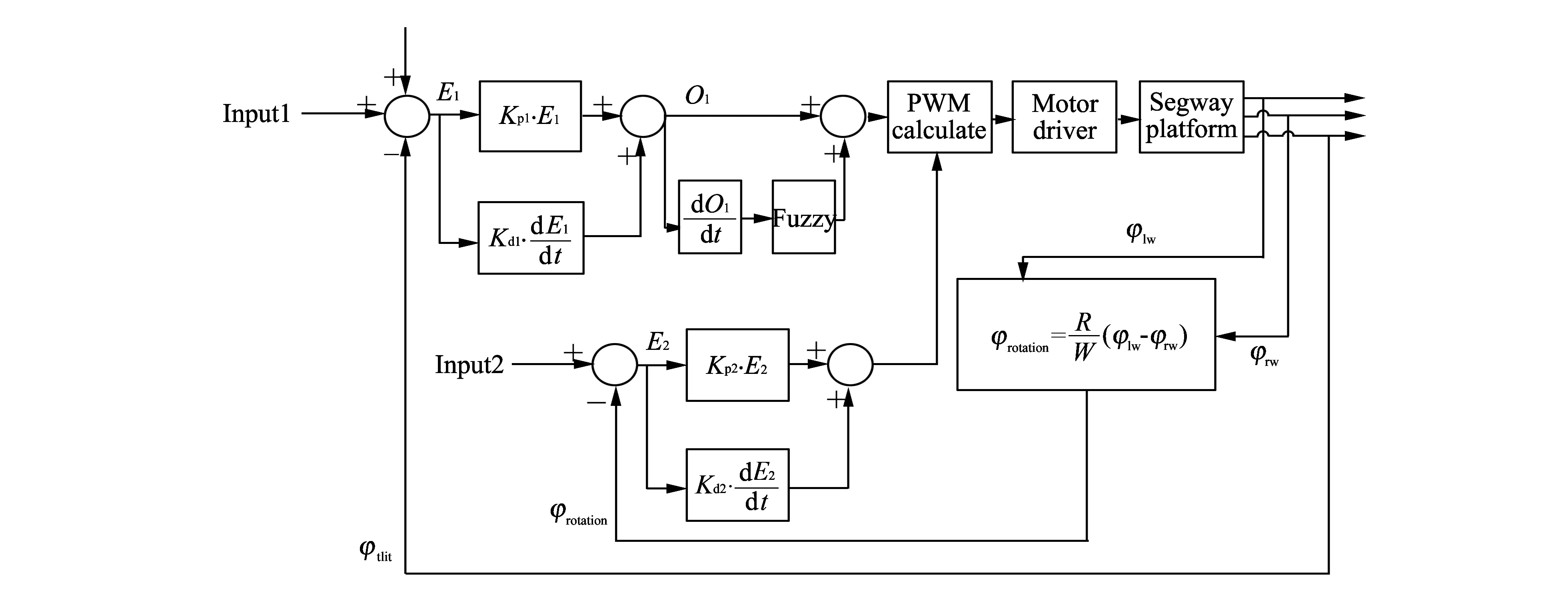
Fig.6 Controller diagram

In Fig.6 input1 is the desired tilt angle for platform without manipulator. Input2 is the desired rotation angle produced by difference of both sides. To keep the robot balance, input1 and input2 are set to be zero. Rotation angle can be got as

where φlwand φrwmean the rotation of left and right wheel, respectively. r is the radius of one wheel and W is the distance of both wheels.

The first PD controller is used to control tilt angle of platform to keep the robot balance and the second PD controller is used to keep both sides move the same distance.

In Fig.6, a fuzzy controller is used to compensate the output of the first PD controller so that the output will not change sharply.

Fuzzy controller receives the differential of O1as its input, where O1is output of the first PD controller. Both IF-THEN rule and rule table of fuzzy controller are used to determine the compensation quantity. Fuzzy membership is shown in Fig.7.

Fig.7 Fuzzy membership

Table 3 is the fuzzy rule, where ph, pb, pm, ps, 0, ns, nm, nb, nl, nh are positive huge, positive large, positive big, positive medium, positive small, zero, negative small, negative medium, negative big, negative large, negative huge.

Table 3 Fuzzy rule

Output of fuzzy controller is defined as

4.3 Experimental results

From the simulation results, compensatory angle is easily got. When the manipulator only moves its first two joints, the minimum compensatory angle is

-0.18×180/π=-10.31°.

(36)

And the maximum compensatory angle is

0.259×180/π=14.84°.

(37)

When the manipulator only moves its and fourth joints of one arm, the compensatory angle are from -3.03° to 10.52°.

In fact, in this experiment, all the joints only change from 0° to 90°, which is enough to check the method. Fig.8 shows the experiment results about the first joint of both arms. From 10 to 40 s, θl1transfers from 0 to 90°, and then from 50 to 80 s θr1transfers from 0 to 90°. Experiment results show that the platform can still keep balance by using compensatory angle. Still, it has the displacement of 1.5 cm and 2.7 cm for left and right side with a body rotation angle about 1.09°.

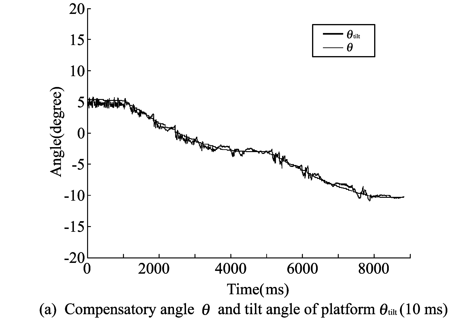
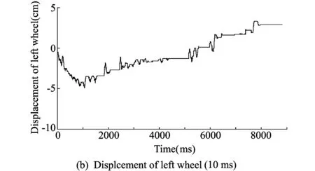
Fig.8 Experiment about the first joint of both arms

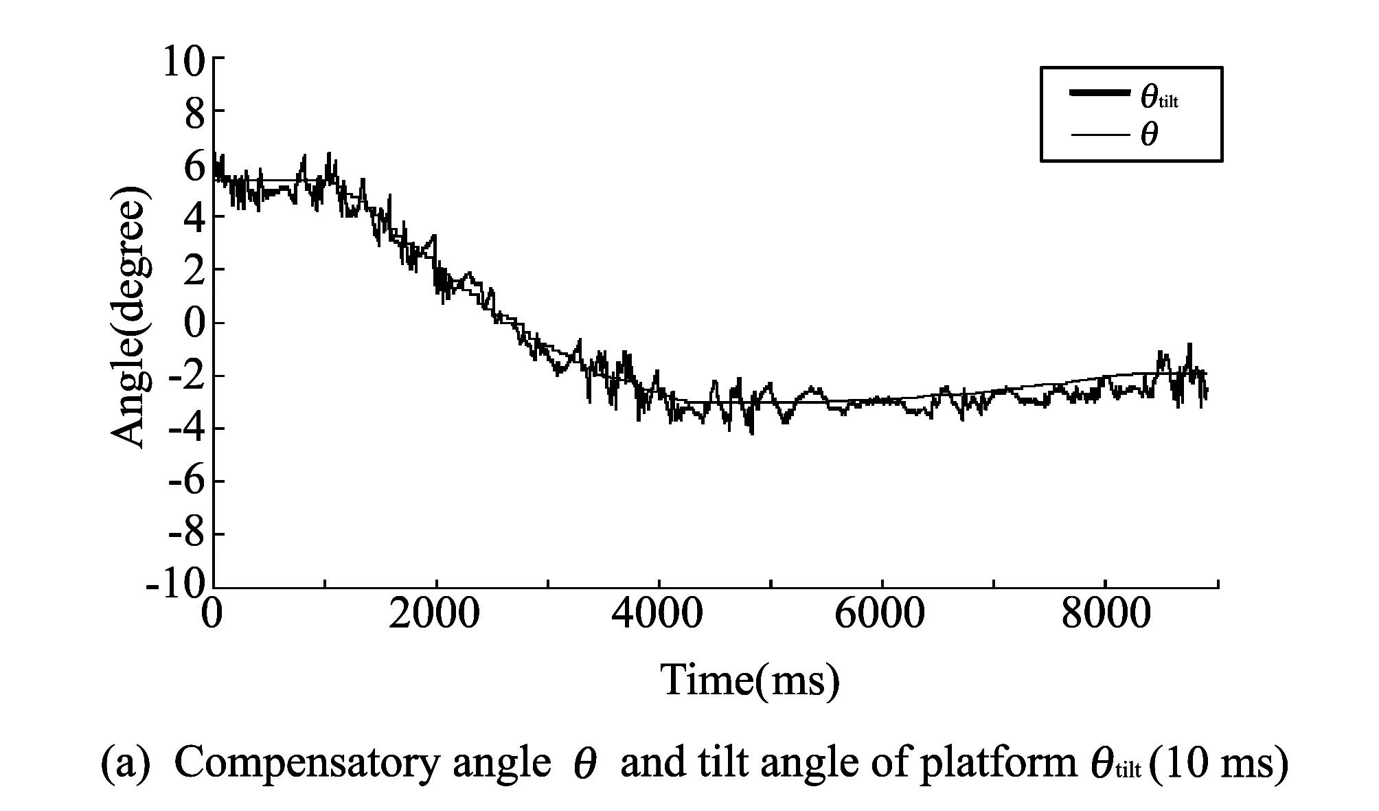
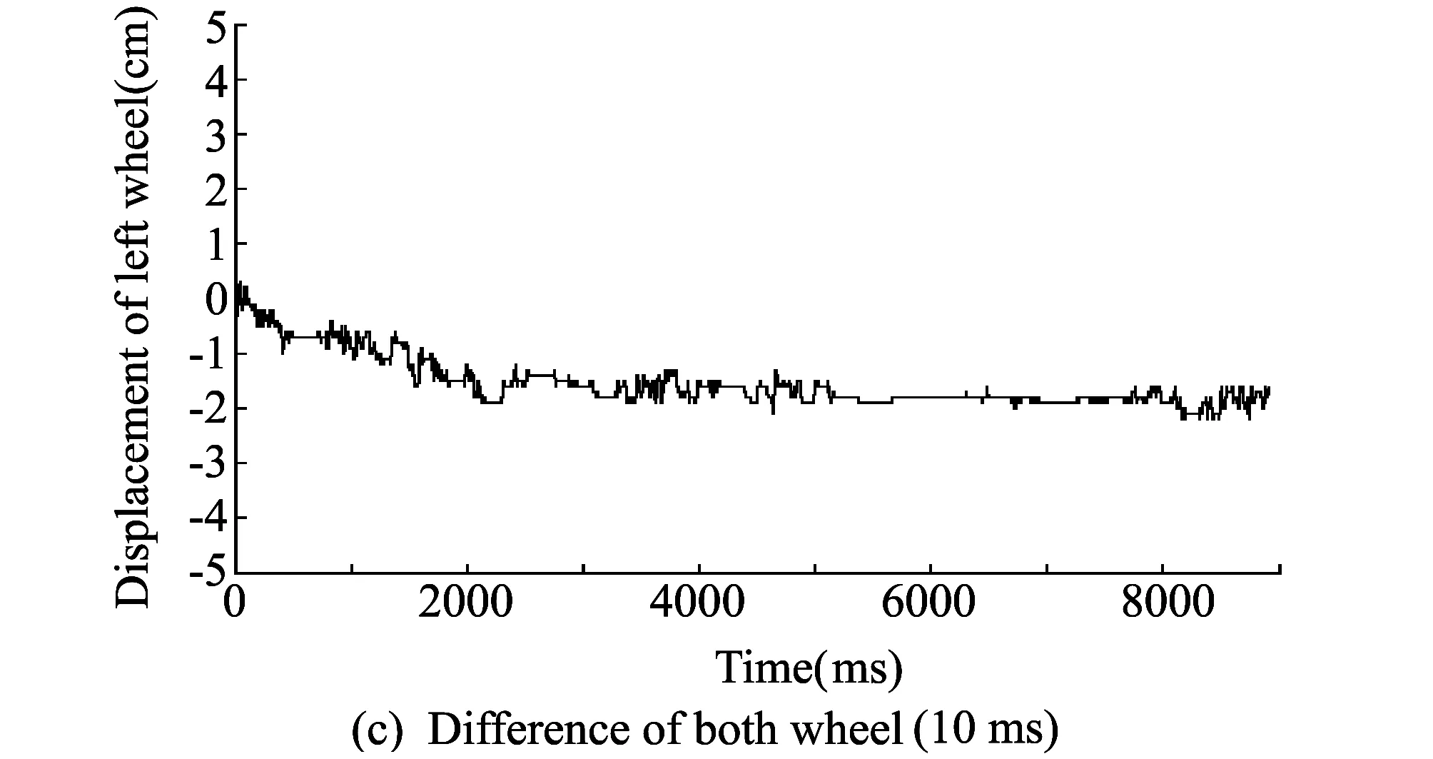
Fig.9 Experiment about the first and the fourth joint of left arm

Fig.9 shows the experiment results about the first and the fourth joint of left arm. From 10 to 40 s, θl1transfers from 0° to 90°, and then from 50 to 80 s, θl4transfers from 0° to 90°. Experiment result shows the similar data as shown in Fig.7.

5 Conclusion

This paper presents a method to control the balance of a mobile manipulator based on two-wheel inverted pendulum robot. By using compensatory angle, the robot can keep balance. As coordinate transformation is widely used in robot engineering, this method is also useful for other similar manipulator which is based on two wheel inverted pendulum robot.

[1] Yamamoto Y, YUN Xiao-ping. Coordinating locomotion and manipulation of a mobile manipulator. IEEE Transactions on Automatic Control, 1994, 39(6): 1326-1332.

[2] Khatib O, Yokoi K, Chang K, et al. Vehicle/arm coordination and multiple mobile manipulator decentralized cooperation. In: Proceedings of 1996 IEEE/RSJ International Conference on Intelligent Robots and Systems, 1996, 2: 546-533.

[3] Yamamoto Y, Eda H, YUN Xiao-ping. Coordinated task execution of a human and a mobile manipulator. In: Proceedings of IEEE International Conference on Robotics and Automation, 1996, 2: 1006-1011.

[4] Nguyen H G, Morrell J, Mullens K, et al. Segway robotic mobility platform. In: SPIE Proceedings 5609: Mobile Robots XVII, Philadelphia, PA, 2004.

[5] Acar C, Murakami T. Multi-task control for dynamically balance two-wheeled mobie manipulator through task-priority. In: Proceedings of 2011 IEEE International Symposium on Industrial Electronics(ISIE), 2011: 2190-2200.

[6] Hosoda Y, Egawa S, Tamamoto J, et al. Basic design of human symbiotic robot EMIEW. In: Proceedings of 2006 IEEE/RSJ International Conference on Intelligent Robots and Systems, 2006: 5079-5084.

date： 2012-09-14

The MKE(the Ministry of Knowledge Economy), Korea, under the Human Resources Development Program for Robotics Support Program supervised by the NIPA(National IT Industry Promotion Agency) (NIPA-2012-H1502-12-1002); the MKE, Korea, under the ITRC(Information Technology Research Center) Support Program supervised by the NIPA (NIPA-2012-H0301-12-2006)

Jangmyung Lee(jmlee@pusan.ac.kr)

CLD number： TP241 Document code： A

1674-8042(2013)01-0052-06

10.3969/j.issn.1674-8042.2013.01.012