An improved ant colony algorithm and its application in optimal routing problem

SONG Jin-juan (宋锦娟)，BAI Yan-ping (白艳萍)

(Dept. of Mathematics, North University of China, Taiyuan 030051, China)

An improved ant colony algorithm and its application in optimal routing problem

SONG Jin-juan (宋锦娟)，BAI Yan-ping (白艳萍)

(Dept. of Mathematics, North University of China, Taiyuan 030051, China)

Ant colony system (ACS), a kind of ant colony algorithm, is an effective way of solving shortest path problem, however, it has some defects. In this paper, ACS is improved for avoiding getting stuck in a local minimum, whose defects mainly include the following two aspects: initial pheromone solution and pheromone updating. In order to learn the advantages of improved ant colony system (IACS), experiments are conducted for some times. First, it is applied to 8 traveling salesman problem (TSP) instances, and compared with three self-organizing map (SOM) algorithms. Then the author analyzes the space complexity and convergence of two algorithms and compares them. Simulation results show that IACS has much better performance in solving TSP, and it has certain theoretical reference value and practical significance.

ant colony system (ACS); pheromone; traveling salesman problem; spcae complexity

0 Introduction

The traveling salesman problem (TSP)[1]is an important problem and also a hot topic in today’s social studies. It is similar to job-shop scheduling,quadratic assignment problem, all of which can be summarized to combinatorial optimization problem. There are many heuristic intelligent algorithms for solving TSP, such as genetic algorithm(GA)[2], simulated annealing (SA)[3], self-organizing map (SOM)[4,5], ant colony algorithm(ACA)[6,7], and so on.

The intelligent algorithm ACS, a kind of improved ACA, has many characteristics such as parallelism, positive feedback and collaboration, however, it still easily gets stuck in a local minimum. So in this paper, an improved ant colony system (IACS) is presented. A new way of calculating initial pheromone value is proposed and ACS global updating rule is adjusted, in which, in addition to the globally shortest path, the pheromone in globally longest path is also updated. Furthermore, the max-min ant system[8]is introduced to effectively stagnation phenomenon caused by great difference of pheromone between the shortest path and the longest path, which can improve the global searching range and avoid local minimum.At last, the rationality and validity of IACS are verified through computer simulation.

1 Description of TSP

The traveling salesman problem is a well-known NP-hard combinatorial optimization problem. TSP[1,9-11]is described as follows: Given a set of N cities, there is a salesman who tries to find the shortest closed path to visit the above N cities under the condition that each city is visited exactly once. It can also be described mathematically as follows: let C be a collection of N cities, where C={c1,c2,…,cN}; and d(ci,cj)∈R+stands for the distance between two cities, where ci,cj∈C(1≤i, j≤N). To achieve a city sequence {cω(1), cω(2), …, cω(N)} under the condition that it makes objective function

be the smallest, where ω(1)，ω(2)，… , ω(N) is a full array of 1,2,…,N.

2 Model of ACS

In ACS, while building a path of TSP, ants can visit edges and change their pheromone level by using the local updating rule. Once all ants have completed their paths, the pheromone level is updated by using the global updating rule.

2.1 ACS state transition rule

In ACS, the state transition rule can be described as follows: an ant positioned on node i chooses the city j to move to using the rule given by

2.2 ACS local updating rule

After choosing a city (that means to visit a edge), the pheromone level of this edge is updated by the local updating rule:

where ξ∈[0,1] is the local pheromone decaying parameter, and τ0is the initial pheromone concentration value of all edges.

2.3 ACS global updating rule

When all ants have completed their closed paths, only the globally best ant who builds the shortest path from the beginning of the trial is allowed to deposit pheromone. The pheromone level is updated by the global updating rule:

where

where ρ∈(0,1) is global pheromone decaying parameter, Δτijis pheromone increment of edge in this circulation, and Lgbis the length of the globally optimal path found so far.

3 IACS

The ACS is an improved ant colony optimization algorithm, the performance of which is improved remarkably, and it is greatly effective in solving TSP and other shortest path problems. However, it still easily gets stuck in a local minimum, so in this paper, some respects must be discussed in the following.

3.1 Way of getting initial pheromone

3.2 Pheromone updating rule

In ACS, only the pheromone in globally shortest path is allowed to be updated, but in this paper, in addition to the globally shortest path, the pheromone in globally longest path is also updated. The pheromone updating rules in globally shortest and longest path are expressed as

where ρ is the global pheromone decaying parameter, Lbestand Lworstare the length of the shortest and longest path, respectively.

3.3 Max-min pheromone system

After pheromone being updated, in order to effectively suppress stagnation phenomenon caused by great difference of pheromone between the shortest and the longest path, the pheromone in every edge is limited in a range [τmin,τmax][8], where τmin=10， τmax=0.0001.

4 Steps of IACS

The steps of IACS are represented as follows:

Step 1: Parameter initialization

Different parameter settings have different influence on experimental results of algorithm, so some experiments are conducted by setting a large number of different parameters, and ultimately the optimal parameter combination is got: α=1，β=2，ζ=0.5，ρ=0.6，q0=0.9， m=5，MaxNc=5 000, where MaxNc represent the maximum number of iteration.

Step 2: Finding the optimal path

In this paper, a set of m ants are placed on n starting nodes (n cities) randomly, and the starting nodes which have been visited by ants are placed in the current solution set tabuk. Each ant will visit the next city j by applying the state transition rules Eqs.(2) and (3), then j is also placed in the current solution set tabuk.

Step 3: Pheromone local updating

The pheromone in the paths!that ants have passed is updated by local updating rule, Eq.(4), then it is determined whether pheromone τij(where τijis the pheromone of path ) is contained in the range [τmin,τmax], if τij>τmax, let τij=τmax; if τij<τmin, let τij=τmin; otherwise, let τijbe itself.

Step 4: Repeating step 2 and 3 until all ants complete their closed path.

Step 5: After iterations of the above four steps, there will be m closed paths, comparing the lengths of m paths, the optimal solution and the worst solution are got and stored. Then the pheromone in the shortest path and the longest path is updated by Eqs.(7) and (8).

Step 6: A set of m ants are placed on n starting nodes (n cities) randomly again, according to step 2, 3 and 4 for optimization, which is repeated, until the 1 000 iterations.

Step 7: The program of path optimization ends until the number of iterations reaches the maximum value. Comparing with the 1 000 optimal solutions of 1 000 iterations, the globally optimal solution will be got, which is also the optimal solution of this algorithm searching for.

5 Experimental results

In order to verify the validity of IACS, 8 examples (such as lin105,ch130, ch150, rat195 and KroA200,etc.) obtained from the general TSPLIB[12]are adopted for experiments. For each example, it is conducted for 10 times, and then the best, average value and the relative error. The experimental results are shown in are calculated, respectively Table 1 and Table 2.

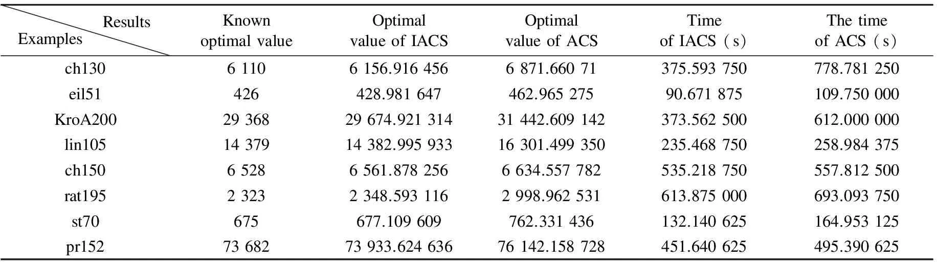
Table 1 Comparison of the best value and time of two algorithms for 10 times

Table 2 Comparison of the average value and relative error of two algorithms

The above comparison of experimental results shows that the optimal value and average value obtained by the improved algorithm are greatly better, and relative error is much smaller than that of ACS, so the improved algorithm introduced in this paper is an effective algorithm. The following diagrams are the experimental results of the improved algorithm. (x stands for longitude, Y stands for latitude, and the unit for each of them is radian.)

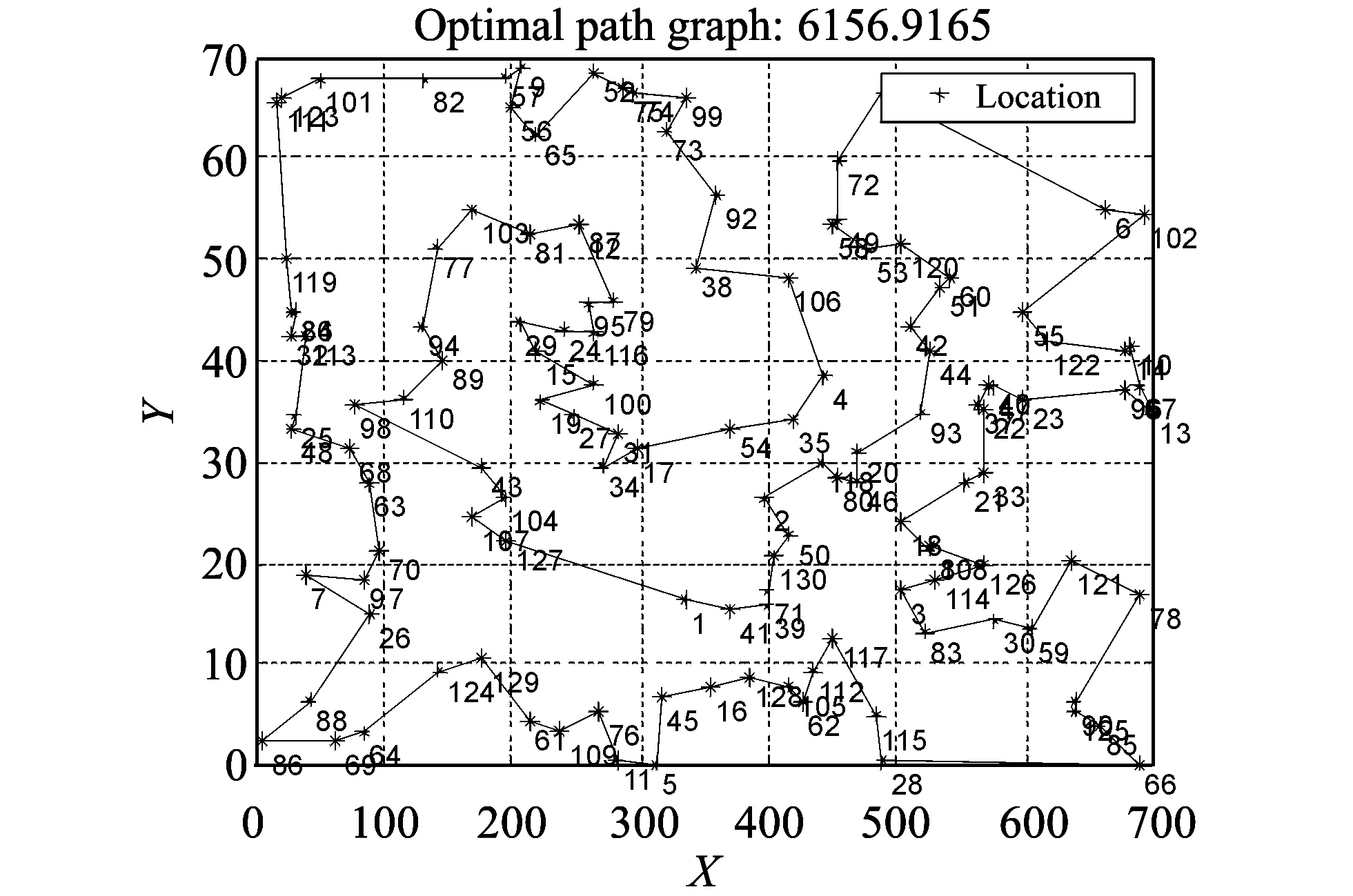
Fig.1 Optimal path graph of ch130

Fig.2 Optimal path graph of eil51

Fig.3 Optimal path graph of KroA200

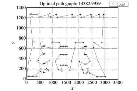
Fig.4 Optimal path graph of lin105

Fig.5 Optimal path graph of ch150

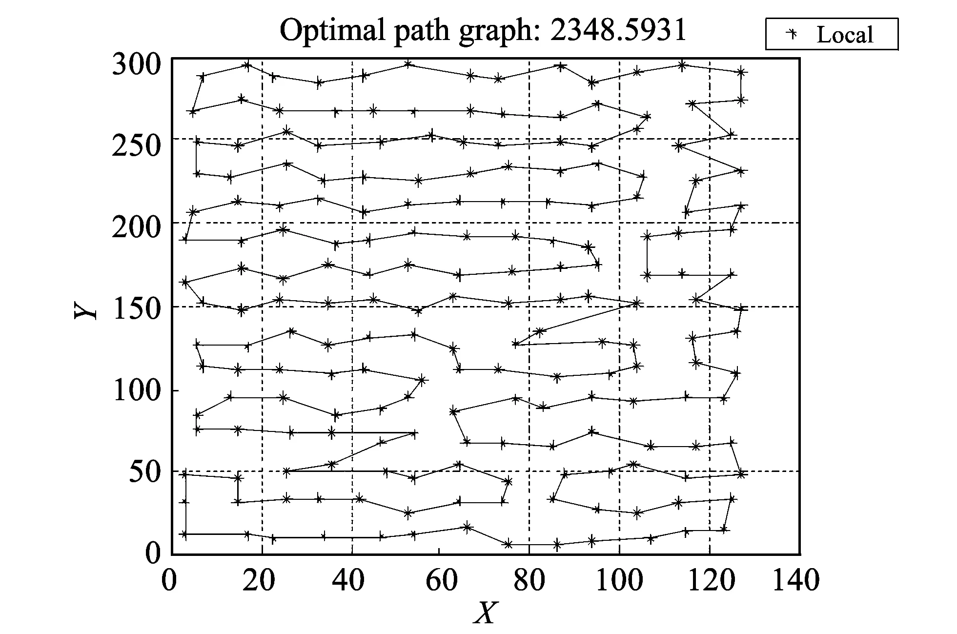
Fig.6 Optimal path graph of rat195

Fig.7 Optimal path graph of st70

Fig.8 Optimal path graph of pr152

In order to further verify the fact that the improved algorithm has better performance, the results obtained by the improved algorithm are compared with that by three kinds of SOM algorithms: Favata-Walke Algorithm (F-W), non-corrdinate self-organizing may (NCSOM) and asymmetric self-organizing map (ASOM)[13]. The comparison results are shown in Table 3.

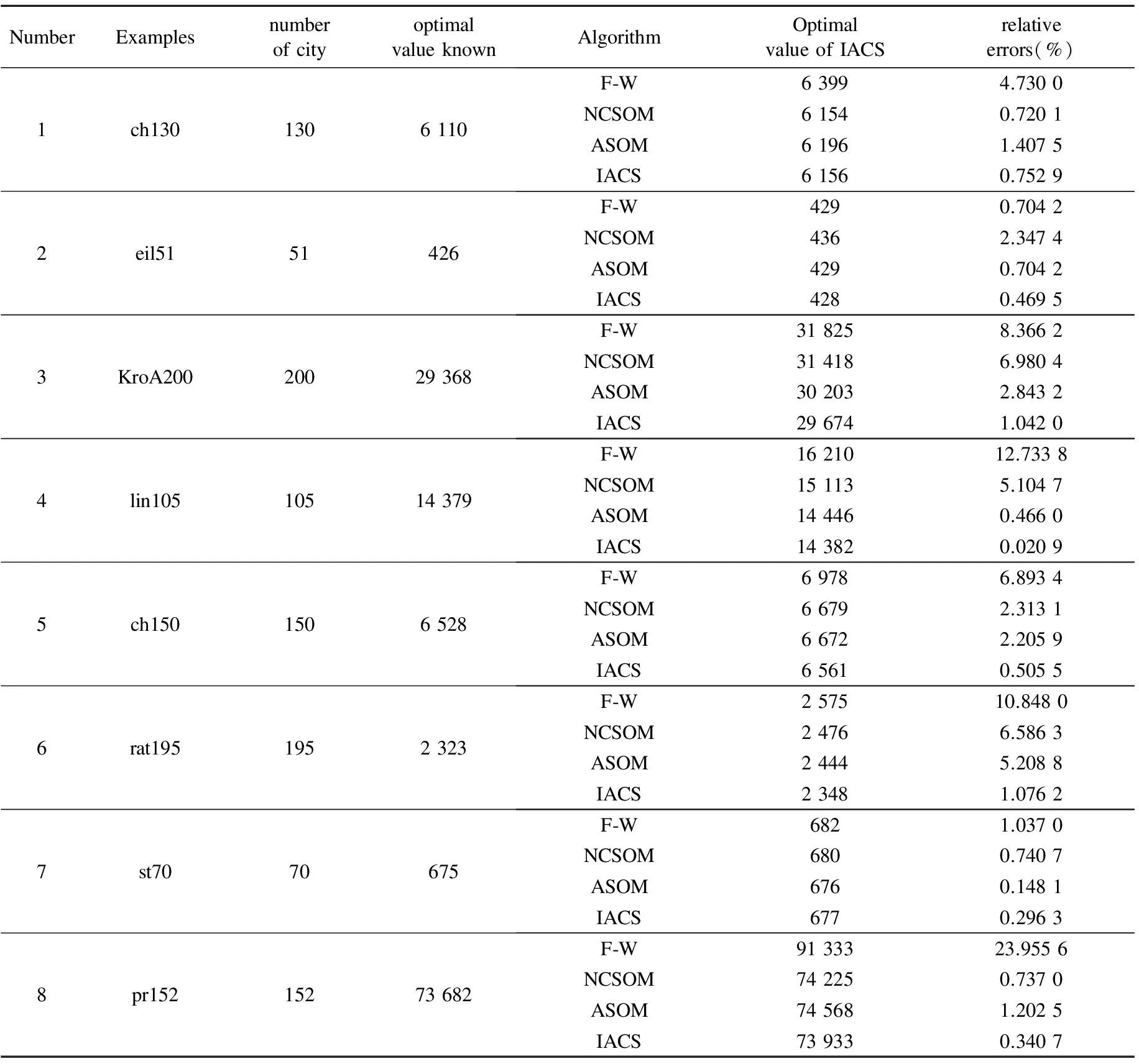
Table 3 Comparison results of four algorithms

From Table 3, it can be seen that for each example of TSP, the experimental results of the improved algorithm are greatly better than other three algorithms. And every optimal value obtained is almost close to the known optimal value.

Finally, the author takes Chinese 34 cities-TSP, a practical problem, for example and makes a comparison between ISOM and ACS based in optimal pathing values and the time. Table 4 and Table 5 show the coordinates of Chinese 34 cities and the comparison of the results of two algorithms, respectively.

Table 4 Coordinates of Chinese 34 cities

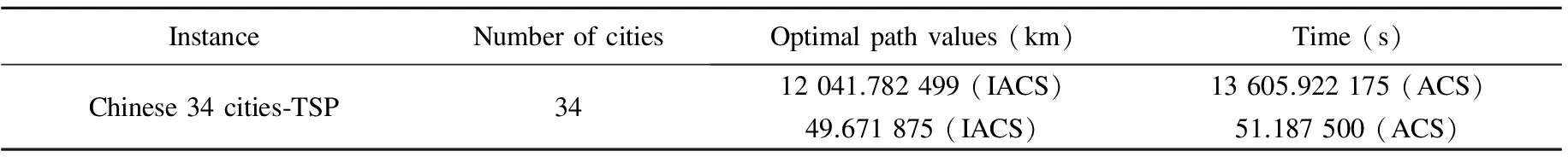
Table 5 Comparison of the results of two algorithms

For the instance Chinese 34 cities-TSP, the optimal path graphs and their corresponing schematic diagrams of variation of global optimal path for two algorithms are shown in Figs.9-12.

Fig.9 Diagram of variation of global optimal path for IACS

Fig.10 Optimal path graph for IACS

Fig.11 Diagram of variation of global optimal path for ACS

Fig.12 Optimal path graph for ACS

6 Algorithm complexity and convergence

Consindering the space complexity of algorithm, we need to analyse the data applied to the algorithm in the process of realization. The data mainly come from two aspects: the description of the problem and the auxiliary data for the realization of algorithm. Taking TSP for example, first, if the scale of TSP is n, we need a n-dimensional two order distance matrix describing the characteristics of the problem itself. For ACS, another n-dimensional two order matrix is needed to describe pheromone concentration of globally shortest path for each iteration. Then, in the process of searching for optimal solution, a n-order one-dimensional matrix is required to establish a tabu list for each ant in order to ensure that the cities visited are no longer chosen in one iteration. In conclusion, we can easily find that the space complexity of ACS algorithm for each iteration may be evaluated as follows: O(n×n)+O(M×n), where M is the number of ants. In IACS algorithm, two n-dimensional two-order matrices are required to describe pheromone concentration of global shortest path and longest path, respectively, so the space complexity of IACS algorithm for each iteration may be evaluated as: O(n×n×n)+O(M×n).

From the comparison between Figs.17 and 19, we can find that ISOM almost reaches the global optimal value when the 600th iteration, while SOM has not reached the global optimal value when the 2 500th iteration. In summary, in spite of a litter higher space complexity of IACS, it has a faster convergence and can achieve better quality results than ACS.

7 Conclusion and discussion

This paper proposes a kind of improved intnlligent ant colony optimization algorithm based on the ACS easily falling into a local optimum, and introduces a kind of new pheromone updating rule and the max-min pheromone system, which makes the ability of the ACS in searching for the globally optimal pth stronger. From the experimental results above, it can easily be found that the improved algorithm has very good searching ability in TSP. However, from Table 1, it can be found that the time of two algorithm is greatly long, which is a aspect need to be improved in the future.

[1] Balachandar S R, Kannan K. Randomized gravitational emulation search algorithm for symmetric traveling salesman problem. Applied Mathematics and Computation, 2007, 192(2): 413-421.

[2] Goldberg D E. Genetic algorithms in search, optimization and machine learning. Addison-Wesley, Boston, 1989.

[3] Van Laarhoven P J, Aarts E H. Simulated annealing: theory and applications. Springer, 1987.

[4] Kohonen T. Self-organized formation of topologically correct feature maps. Biological Cybernetics, 1982, 43(1): 59-69.

[5] Fort J C. Solving a combinatorial problem via self-organizing process: an application of the Kohonen algorithm to the traveling salesman problem. Biological Cybernetics, 1988, 59(1): 33-40.

[6] Dorigo M, Gambardella L M, Ant colony system: a cooperative learning approach to the traveling salesman problem, IEEE Transactions on Evolutionary Computation, 1997, 1(1): 53-56.

[7] Mullen R J, Monekosso D, Barman S, et al. A review of ant algorithms. Expert Systems with Applications, 2009, 36 (6): 9608-9617.

[8] Stützle T, Hoos H H. Max-min ant system. Future Generation Computer Systems, 2000, 16(8): 889-914.

[9] ZHANG Wen-dong, BAI Yan-ping, HU Hong-ping. The incorporation of an efficient initialization method and parameter adaptation using self-organizing maps to solve the TSP. Applied Mathematics and Computation, 2006, 172(1): 603-623.

[10] CHENG Chi-bin, MAO Chun-pin. A modified ant colony system for solving the traveling salesman problem with time windows. Mathematical and Computer Modelling, 2007, 46(9/10): 1225-1235.

[11] Yadlapalli S, Malik W A, Darbha S, et al. A lagrangian-based algorithm for a multiple depot, multiple traveling salesmen problem. Nonlinear Analysis: Real World Applications, 2009, 10(4): 1990-1999.

[12] Ruprecht-karls-universitat heidelberg. Symmetric traveling salesman problem (TSP): TSP data, best solutions for symmetric TSPs. [2012-08-15]. http://www.iwr.uni-heidelberg.de/groups/comopt/software/TSPLIB95/.

[13] WU Ling-yun. The application for neural networks in combinatorial optimization and DNA sequencing. Department of Mathematics, Academy of Sciences, China, 2002: 51-56.

date： 2012-09-30

National Natural Science Foundation of China (No.61275120)

SONG Jin-juan (jinjuansong666@163.com)

CLD number： TP301.6 Document code： A

1674-8042(2013)01-0023-07

10.3969/j.issn.1674-8042.2013.01.006