Modeling of Surface Tension and Viscosity for Non-electrolyte Systems by Means of the Equation of State for Square-wellChain Fluids with Variable Interaction Range*

LI Jinlong (李进龙), HE Changchun (何昌春), MA Jun (马俊), PENG Changjun (彭昌军)**,LIU Honglai (刘洪来) and HU Ying (胡英)

State Key Laboratory of Chemical Engineering and Department of Chemistry, East China University of Science and Technology, Shanghai 200237, China

1 INTRODUCTION

It has been long recognized that the equations of state (EOS) can be extensively used for descriptions of thermodynamic properties such as phase equilibrium,surface tension, viscosity, and caloric properties [1, 2].So far, many EOSs have been developed for calculations of various physicochemical properties. One of the most successful EOSs is the statistical associating fluid theory (SAFT), first proposed by Chapman et al.[3, 4] about two decades ago. After that, many derived versions of SAFT-based EOSs have been presented and several detailed reviews have been made [1, 2, 5, 6].In SAFT, the special point is to capture both the chain length (molecular size and shape) and the molecular association for a reference fluid in place of the simple hard sphere reference fluid while the effects due to other interactions such as dispersion, induction, and polar are brought into a perturbation term. Coupling with density functional theory, density gradient theory,or scaled particle theory, the SAFT related EOSs have been satisfactorily extended to study the surface tension and viscosity of common pure fluids and mixtures [1]. Recently, Wang et al. [7] presented a comprehensive model, which is a combination of a correlation for computing the surface tension of solvent mixture and a formula for the influence of electrolyte concentration and can be used for complex electrolyte systems ranging from dilute solutions to fused salts.Some experimental data for surface tension and viscosity of ionic liquid (IL) related systems have been reported [8-14], but SAFT based EOS is seldom used to model the properties. Thus, in the present work, we will compute the surface tension and viscosity of IL related systems and common fluids by combining a new EOS, which was recently developed in our laboratory [15], the scaled particle theory [16], and a viscosity model [17]. In the EOS, two modifications for dispersion and chain formation terms have been made:(1) a new square well dispersion term with variable interaction range (1.1≤λ≤3) is derived, and (2) the chain formation term is divided into the hard sphere chain formation contribution and the effects of square well dispersion on chain formation of hard spheres.The residual Helmholtz free energy of a mixture is written as [15]

where the superscripts hs-mono, sw-mono, hs-chain,and sw-chain represent the contributions from hard sphere monomers, square well dispersion, the formation of hard chain, and the effects of square well potential on the formation of hard chain, respectively. In the model, each molecule is characterized by four molecular parameters, namely, segment number (r),segment diameter (σ), dispersion interaction energy (ε)and reduced well width (λ). The SWCF-VR EOS can well reproduce the vapor-liquid coexistence curves and the compressibility factor of prototype fluids as well as real fluids [5, 16, 18-21]. The salient feature is that the molecular parameters in this model are selfconsistent and can be obtained by fitting the experimental saturated pressure and/or liquid volume data.

2 BRIEF DESCRIPTION OF MODELS FOR SURFACE TENSION AND VISCOSITY

2.1 Surface tension

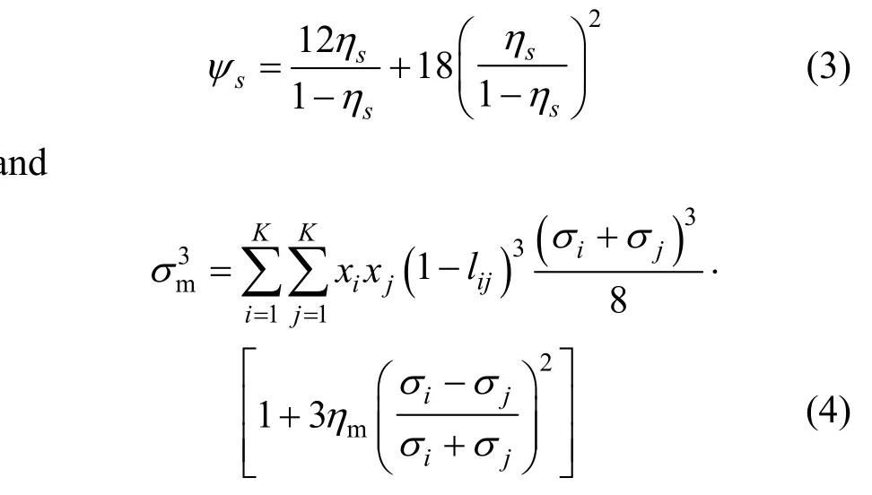
Based on the scaled particle theory (SPT) [22], a vapor-liquid interfacial tension model for liquid mixture has been presented and the formula is [16]where γ is the surface tension, σ is the segment diameter, x is the mole fraction of liquid component, K is the number of component in a mixture, the subscripts i and m repesent the pure component i and a mixture, respectively. In Eq. (2),=m,siψ and σmare calculated as follows a where lijis the adjustable size parameter. The reduced density of a mixture in Eqs. (3) and (4), ηm, can be obtained with any EOS by the relationship where R is the gas constant, r is segment number of pure component i, p and T denote system pressure and temperature, z is the compressibility factor of a mixture and can be calculated with SWCF-VR EOS [15].In calculating the compressibility factor, the crossing segment diameter (σij) and well depth (εij) are estimated through the standard Lorentz-Berthelot rules [23] as

respectively. For the unlike interaction square-well potential range parameter λij, a simple arithmetic combining rule is used

In Eq. (7), κijis an adjustable energy parameter. Note that the crossing segment diameter in calculation of compressibility factor of a mixture is always given by Eq. (6) and no binary interaction parameter is used.

2.2 Viscosity

Based on Eyring’s viscosity theory at elevated pressure, Xuan et al. [17] presented a viscosity model for pure fluids

where μ is the viscosity, k1and k2denote the adjustable model parameters, and z is the compressibility factor which can be calculated with SWCF-VR EOS.In the model, the effect of temperature on viscosity is characterized by k1, k2and z, and the effect from pressure is only depicted by z. The details of this model are described in Xuan et al.’s work [17].

3 RESULTS AND DISCUSSION

To calculate the surface tension and viscosity, it is necessary to know the model parameters of pure fluids. These molecular parameters for various pure fluids has been obtained through fitting the experimental saturated vapor pressure and/or liquid volumetric values in our previous work [18, 19] and listed in Table 1 for the fluids investigated in this work.Once the model parameters are given, it is convenient to calculate the surface tension and viscosity on the basis of the given models. To improve the calculated precision of surface tension and determine the adjustable parameters (k1and k2) in viscosity model, an objective function is used

where Npis the number of experimental data point, θ represents the surface tension or viscosity, superscripts exp and cal denote the experimental and calculated results respectively.

3.1 Surface tension

The detailed calculation process for the surface tension is as follows. The compressibility factor of pure fluid and mixture at given temperatures and pressures is first calculated using SWCF-VR EOS [15].The reduced density of a mixture is given by Eq. (5).The parameters ψmand σmare then computed withEqs. (3) and (4) respectively. Finally, the surface tension of a mixture under given condition is obtained from Eq. (2). To improve the calculation precision,bothlijandκijor either of them are considered as adjustable parameters and obtained by fitting the experimental surface tension.

Table 1 Molecular parameters for the pure substances investigated

Table 2 The predicted and correlated results of surface tension for binary mixtures

Table 2 (Continued)

3.1.1Correlations

The correlated results and adjustable parameters in 24 cases for 18 binary mixtures are listed in Table 2,with the sources of experimental values. The overall average relative deviation, except for IL mixtures, is 2.56% for prediction withκij=lij=0, 0.42% for correlation withκij, 0.41% for correlation withlij, and 0.36% for correlation with bothκijandlij. The calculation precision of surface tension can be greatly improved when using adjustable parameter eitherκijorlij,and the improvement is almost the same with the correlated values ofκijandlij. Thus, one adjustable parameter (eitherκijorlij) is recommended to use for practical applications. A typical graphical comparison between theoretical calculations and experiments for cyclopentane(1) + benzene(2) [32] and hexane(1) +acetone(2) [33] mixtures is illustrated in Fig. 1. The calculated results with adjustable parameterlijwell agree with experimental values.

To test the feasibility of this model for mixtures containing ILs, two typical examples [8] are given in this work, as illustrated in Fig. 2. The results are satisfactory with one adjustable parameterκij. However,the deviations increase at low IL concentrations for[C4mim][NTf2] + 1-butanol mixture. The reason may be that the associations of alcohols and the long rang static interactions of ILs are not considered in this model.

Figure 1 Comparison of theoretical (lines) and experimental [32, 33] (symbols) surface tension of mixtures (solid line:correlation with lij; dash line: predicted with κij=lij=0)□ cyclopentane(1) + benzene(2); ○ n-hexane(1) + acetone(2)

Based on SPT, Liet al. [42] also proposed a model for surface tension of liquid mixtures. In the model, a real mixture is supposed as a pseudo-pure fluid and the expression is written as

Figure 2 Comparison of theoretical (lines) and experimental [8] (symbols) surface tension of IL mixtures (solid lines: correlations; dash lines: predictions)

Table 3 Predicted surface tension of bianry mixtures at different temperatures

whereγmdenotes the surface tension of the mixture,σma pseudo-dimeter andηmthe reduced density. In this model, a new molecular parameterσis first determined by fitting the experimental surface tension and liquid density of pure fluid. The pseudo-diameterσmis then obtained by combining a cross rule (such as Meyer’s cross rule [43]). Finally, the surface tension for a mixture is calculated by Eq. (11). The calculation accuracy of our model and Liet al.’s equation for eight mixture systems (cyclohexane +n-hexane,cyclohexane + chlorobenzene, tetrachloromethane +benzene,n-hexane + acetone, benzene + acetone,cyclopentane + toluene, cyclopentane + tetrachloromethane and toluene + ethyl acetate) that are random selected is obtained and the overall average deviations are 0.40% and 0.42%, respectively. In calculations,only one adjustable parameterlijin Eq. (4) is used to improve the correlation precision in both models.However, in Liet al.’s model [42] a real fluid is supposed to be composed of sphere molecules and a new molecular parameterσis required and obtained from the experimental surface tension and liquid density for calculating surface tension of the mixture. A real fluid molecule in this model is a chain molecule composed ofrsegments with a diameter ofσ, and the molecular parameters used in our model are self-consistent and can be applied for calculations of vapor-liquid equilibrium, caloric properties, surface tension,etc.

3.1.2Predictions

Parametersκijandlijlisted in Table 2 for a given mixture are almost identical at different temperatures,indicating that the surface tension of a binary mixture at other temperatures can be predicted afterκijorlijis obtained from experimental values at a specific temperature, for example, at room temperature. The surface tensions for several typical binary mixtures are predicted with the binary interaction parameterκijorlijdetermined from the experimental surface tension at 293.15 K, as shown in Table 3 and Fig. 3 (a). The predicted results are in good agreement with experiments[40]. In addition, the surface tension of multicomponent mixtures can be predictedviathe binary adjustable parameter, as shown in Fig. 3 (b). Good consistency between the theoretical predictions withκijand the experimental surface tension for two ternary mixtures [33, 34] is obtained.

Figure 3 Comparison of the predicted and experimental [33, 34, 40] surface tension for mixtures

Table 4 Calculated results of viscosity at high pressure for common fluids and ionic liquids

Table 4 (Continued)

Table 4 (Continued)

3.2 Viscosity

In the viscosity model, two adjustable parametersk1andk2are determined based on the experimental viscosity data. The calculation process is as follows.The molecular parameters are obtained by fitting the experimental saturated vapor pressure and liquid volumetric properties. The compressibility factor at a given temperature and pressure are computed using SWCF-VR EOS. The viscosity under a given condition is determined by substituting the obtained compressibility factor to Eq. (9).

This model is employed to calculate the viscosities of 14 pure components in different temperature and pressure ranges and the results are listed in Table 4,with the adjustable parametersk1andk2, the average relative deviations and data sources. The highest pressure for some systems is up to 300 MPa and the overall average absolute deviation is only 1.44%, and the average relative deviations are 2.21% for common fluids and 0.70% for ILs. A graphical comparison between theoretical and experimental [44, 45] viscosities at 303 K for several common alkanes are shown in Fig. 4. The pressure ranges from 0.1 to 250 MPa. The theoretical results are in good agreement with experiments. Another typical comparison between correlations and experiments [11] of viscosity at the temperature range from 298.15 to 348.15 K and pressure up to 200 MPa for ionic liquid [C8mim][BF4] is illustrated in Fig. 5 and good consistency is also observed.

Figure 4 Theoretical (lines) and experimental [44, 45](symbols) results of viscosity at 303.15K for n-alkanes□ n-pentane; ○ n-hexane; △ n-octane; ▽ n-decane

Figure 5 Theoretical (lines) and experimental [11](symbols) results of viscosity at different temperaturesfor[C8mim][BF4]T/K: □ 298.15; ○ 308.15; △ 323.15; ▽ 333.15; ◇ 348.15

Figure 6 Relationship between lg(k1)/lg(k2) and 1/T (symbols: modeled results; lines: drawn to guide the eye)

Table 4 also shows that the logarithm values ofk1and/ork2for common fluids and ILs can be expressed as a linear function of the reciprocal of temperature(1/T),viz.The linear relationships between the logarithm ofk1and 1/Tforn-alkanes are shown in Fig. 6 (a). The logarithms of bothk1andk2have a good linear relationship with 1/Tfor ILs as shown in Fig. 6 (b). Actually, it is not surprising that the logarithm values ofk1is a linear function of 1/Tas the relationship between viscosity of liquid at low pressure and 1/Tcan be written as ln(μ)=A+B/Taccording to Eyring’s viscosity model.For model parameterk2in the viscosity model, it should also have a linear relationship with 1/Tsincek2is proportional to exp( / )EkT≠- , whereE≠is the molecular activation energy. From Table 4, no linear relation is observed for common fluids while a linear relationship exists for some ionic liquids as shown in Fig. 6 (b). The reason may be that the effect ofTonk2is smaller than onk1and the regressed parameter is only an optimum value at different temperatures [17].Furthermore, the obtained values ofk1at a given temperature for all systems are almost equal to the real viscosity data at the corresponding temperature and a pressure of 0.1 MPa, as shown by Xuanet al. [17]. It may be explained as that the compressibility factor of liquid at low pressure is so small that the value of exp(k2z) in Eq. (9) is approximately equal to 1. In addition, it should be stressed that the logarithms of parametersk1andk2at certain temperature for homologousn-alkanes are proportional to their molecular mass. This indicates that the model can be used to predict the viscosity of some homologous compounds under certain condition when no experimental viscosity is available.

4 CONCLUSIONS

Coupled with the scaled particle theory and Xuanet al.’s viscosity model, the equation of state for square well chain fluid with variable interaction range was extended to represent the surface tension of multicomponent liquid mixtures at atmospheric pressure and viscosity of pure substance at elevated pressure.The feasibility of the two models was checked and confirmed for real systems containing common fluids and ionic liquids, and excellent agreement between the theoretical and experimental results was observed.The distinct feature of this model is that the molecular parameters can be used to calculate thepVT, vapor-liquid equilibrium, caloric properties, surface tension, viscosity,etc., indicating that the models can be used for industrial practice.

1 Tan, S.P., Adidharma, H., Radosz, M., “Recent advances and applications of statistical associating fluid theory”,Ind.Eng.Chem.Res.,47, 8063-8082 (2008).

2 Wei, Y.S., Sadus, R.J., “Equation of state for the calculation of fluid-phase equilibria”,AIChE J., 46, 169-196 (2000).

3 Chapman, W.G., Gubbins, K.E., Jackson, G., Radosz, M., “SAFT:Equation of state solution model for associating fluids”,Fluid Phase Equilib., 52, 31-38 (1989).

4 Chapman, W.G., Gubbins, K.E., Jackson, G., Radosz, M., “New reference equation of state for associating liquids”,Ind.Eng.Chem.Res., 29, 1709-1721 (1990).

5 Li, J.L., He, C.C., Peng, C.J., Liu, H.L., Hu, Y., “Equation of state for chain like fluid based on statistical theory for chemical association”,Sci.Chin.Chem., 40, 1198-1209 (2010).

6 Muller, E.A., Gubbins, K.E., “Molecular-based equations of state for associating fluids: A review of SAFT and related approaches”,Ind.Eng.Chem.Res., 40, 2193-2211 (2001).

7 Wang, P., Anderko, A., Young, D.R., “Modeling surface tension of concentrated and mixed-solvent electrolyte systems”,Ind.Eng.Chem.Res., 50, 4086-4098 (2011).

8 Wandschneider, A., Lehmann, J.K., Heintz, A., “Surface tension and density of pure ionic liquids and some binary mixtures with 1-propanol and 1-butanol”,J.Chem.Eng.Data, 53, 596-599 (2008).

9 Ahosseini, A., Scurto, A.M., “Viscosity of imidazolium based ionic liquids at elevated pressures: Cation and anion effects”,Int.J.Thermophys., 29, 1222-1243 (2008).

10 Harris, K.R., Kanakubo, M., Woolf, L.A., “Temperature and pressure dependence of the viscosity of the ionic liquid 1-methyl-3-octylimidazolium hexafluorophosphate and 1-methyl-3-octylimidazolium tetrafluoroborate”,J.Chem.Eng.Data, 51, 1161-1167 (2006).

11 Harris, K.R., Kanakubo, M., Woolf, L.A., “Temperature and pressure dependence of the viscosity of the ionic liquid 1-butyl-3methylimidazolium tetrafluoroborate: Viscosity and density relationships in ionic liquids”,J.Chem.Eng.Data, 52, 2425-2430(2007).

12 Harris, K.R., Woolf, L.A., Kanakubo, M., “Temperature and pressure dpendence of the viscosity of the ionic liquid 1-butyl-3-methylimidazolium hexafluorophosphate”,J.Chem.Eng.Data, 50, 1777-1782 (2005).

13 Tomida, D., Kumagai, A., Kenmochi, S., Qiao, K., Yokoyama, C.,“Viscosity of 1-hexyl-3-methylimidazolium hexafluorophosphate and 1-octyl-3-methylimidazolium hexafluorophosphate at high pressure”,J.Chem.Eng.Data, 52, 577-579 (2007).

14 Tomida, D., Kumagai, A., Qiao, K., Yokoyama, C., “Viscosity of[Bmim][PF6] and [Bmim][BF4] at high pressure”,Int.J.Thermophys., 27, 39-47 (2006).

15 Li, J.L., He, H.H., Peng, C.J., Liu, H.L., Hu, Y., “A new development of equation of state for square-well chain-like molecules with variable width 1.1≤λ≤3”,FluidPhaseEquilib., 276, 57-68 (2009).16 Li, J.L., Ma, J., Peng, C.J., Liu, H.L., Hu, Y., Jiang, J.W., “Equation of state coupled with scaled particle theory for surface tension of liquid mixtures”,Ind.Eng.Chem.Res., 46, 7267-7274 (2007).

17 Xuan, A., Wu, Y., Peng, C.J., Ma, P.S., “Correlation of the viscosity of pure liquids at high pressures based on an equation of state”,Fluid Phase Equilib., 240, 15-21 (2006).

18 Li, J.L., He, H.H., Peng, C.J., Liu, H.L., Hu, Y., “Equation of state for square-well chain molecules with variable range. I: Application for pure substances”, Fluid Phase Equilib., 286, 8-16 (2009).

19 Li, J.L., He, Q., He, C.C., Peng, C.J., Liu, H.L., “Represention of phase behavior of ionic liquids using the equation of state for square well chain fluids with variable range”, Chin. J. Chem. Eng., 17,983-989 (2009).

20 Li, J.L., Peng, C.J., Liu, H.L., “Mdeling vapor-liquid equilibrium of refrigerants using an equation of state for square well chain fluid with variable range”, CIESC J., 60, 545-552 (2009).

21 Li, J.L., Tong, M., Peng, C.J., Liu, H.L., Hu, Y., “Equation of state for square-well chain molecules with variable range. II: Extension to mixture”, Fluid Phase Equilib., 287, 56-67 (2009).

22 Reiss, H., Frisch, H.L., Helfand, E., Lebowitz, J.L., “Aspects of the statistical thermodynamics of real fluids”, J. Chem. Phys., 32,119-124 (1960).

23 Rowlinson, J.S., Swinton, F.L., Liquids and Liquid Mixtures. 3rd ed.;Butterworth, London (1982).

24 Smith, B.D., Srivastava, R., Thermodynamic Data for Pure Compounds, Elsevier, Amsterdam (1986).

25 Daubert, T.E., Danner, R.P., Physical and Thermodynamic Properties of Pure Chemicals, John wiley & Sons, New York (1989).

26 Vargaftik, N.B., Tables on the Thermophysical Properties of Liquids and Gases, John Wiley & Sons, New York (1975).

27 Lu, H.Z., Handbook of Petrochemical Data, Chemical Industry Press,Beijing (1982).

28 Machida, H., Sato, Y., Smith, J.R.L., “Pressure-volume-temperature measurement of ionic liquids ([Bmim][PF6], [Bmim][BF4],[Bmim][OcSO4]”, Fluid Phase Equilib., 264, 147-155 (2008).

29 Gardas, R.L., Freire, M.G., Carvalho, P.J., Marrucho, I.M., Fonseca,I.M.A., Ferreira, A.G.M., COutinho, J.A.P., “High pressure densities and derived themodynamic properties of imidazolium-based ionic liquids”, J. Chem. Eng. Data, 52, 80-88 (2007).

30 Fredlake, C.P., Crosthwaite, J.M., Hert, D.G., Aki, S.N.V.K., Brennecke, J.F., “Thermophysical properties of imidazolium based ionic liquids”, J. Chem. Eng. Data, 49, 954-964 (2004).

31 Azevedo, R.G., Esperanca, J.M.S.S., Szydlowski, J., Visak, Z.P.,Pires, P.E., Guedes, H.J.R., Rebelo, L.P.N., “Thermophysical and thermodynamic properties of ionic liquids over an extended pressure range: [Bmim][NTf2] and [Hmim][NTf2]”, J. Chem. Thermodyn., 37,888-899 (2005).

32 Lam, V.T., Benson, G.C., “Surface tensions of binary liquid systems I. Mixture of nonelectrolytes”, Can. J. Chem., 48, 3773-3781(1970).

33 Rusanov, A.I., Levichev, S.A., “Thermodynamic investigation of surface layers of liquid solutions”, Kolloidn. Zh., 30, 112-118 (1968).

34 Ridgway, K., Bulter, P.A., “Some physical properties of the ternary system benzene + cyclohexane + n-hexane”, J. Chem. Eng. Data, 12,509-515 (1967).

35 Clever, H.L., Chase, M.W., “Thermodynamics of liquid surfaces:Surface tension of n-hexane-cyclohexane mixture at 25, 30 and 35 °C”, J. Chem. Eng. Data, 8, 291-292 (1963).

36 Suri, S.K., Ramakrishna, V., “Surface tension of some binary liquid mixture”, J. Phys. Chem., 72, 3073-3079 (1968).

37 Siskova, M., Secova, V., “Surface tension of binary solution of non-electrolytes V”, Collect. Czech. Chem. Commun., 35, 2702-2711(1970).

38 Koefoed, J., Villadsen, J.V., “Surface tension of liquid mixtures: A micro-method applied to the system: chloroform-carbon-tetrachloride,benzene-diphenylmethane and heptane-hexadecane”, Acta Chem.Scand., 12, 1124-1134 (1958).

39 Waket, E.S., “Surface tension of binary mixtures of several organic liquids at 25 °C”, J. Chem. Eng. Data, 15, 308-311 (1970).

40 Schmidt, R.L., Randall, J.C., Clever, H.L., “Surface tension and density of binary hydrocarbon mixtures”, J. Phys. Chem., 70,3912-3918 (1966).

41 Litkenhous, E.E., van Arsdale, J.D., Hutchison, I. W., “The system butyl alcohol-ehtyl acetate-toluene”, J. Phys. Chem., 44, 377-382(1940).

42 Li, Z.B., Hu, Y.Q., Li, Y.G., Lu, J.F., “Molecular model of vaporliquid and liquid-liquid interface tension for mixture”, Chem. Eng.,28, 57-61 (2000).

43 Meyer, E.C., “A one-fluid mixing rule for hard spheres mixtures”,Fluid Phase Equilib., 41, 19-29 (1988).

44 Kiran, K., Sen, Y.L., “High-pressure viscosity and density of n-alkanes”, Int. J. Thermophys., 13, 411-445 (1992).

45 Oliveira, C.M.B.P., Wakeham, W.A., “The viscosity of five liquid hydrocarbons at pressure up to 250 MPa”, Int. J. Thermophys., 13,773-790 (1992).