Long-Term Extreme Wave Characteristics in the Water Adjacent to China Based on ERA5 Reanalysis Data

DU Wenyan, ZHANG Xuri, SHI Hongyuan, , LI Guanyu, ZHOU Zhengqiao,YOU Zaijin, and ZHANG Kuncheng

1) School of Hydraulic Engineering, Ludong University, Yantai 264025, China

2) Center for Ports and Maritime Safety (CPMS), Dalian Maritime University, Dalian 1160263, China

3) Nation Ocean Technology Center, Tianjin 300111, China

4) Navigation Guarantee Center of South China Sea (NGCS) MOT Guangzhou Hydrographic Center, Guangzhou 510320,China

5) Institute of Marine Development / Military Teaching Department, School of Marxism, Ocean University of China,Qingdao 266100, China

6) Yantai Kekan Marine Technology Co., Ltd., Yantai 264025,China

Abstract Extreme waves have a profound impact on coastal infrastructure; thus, understanding the variation law of risky analysis and disaster prevention in coastal zones is necessary. This paper analyzed the spatiotemporal characteristics of extreme wave heights adjacent to China from 1979 to 2018 based on the ERA5 datasets. Nonstationary extreme value analysis is undertaken in eight representative points to investigate the trends in the values of 50- and 100-year wave heights. Results show that the mean value of extreme waves is the largest in the eastern part of Taiwan Island and the smallest in the Bohai Sea from 1979 to 2018. Only the extreme wave height in the northeastern part of Taiwan Island shows a significant increase trend in the study area. Nonstationary analysis shows remarkable variations in the values of 50- and 100-year significant wave heights in eight points. Considering the annual mean change,E1, E2, S1, and S2 present an increasing trend, while S3 shows a decreasing trend. Most points for the seasonal mean change demonstrate an increasing trend in spring and winter, while other points show a decreasing trend in summer and autumn. Notably, the E1 point growth rate is large in autumn, which is related to the change in typhoon intensity and the northward movement of the typhoon path.

Key words extreme wave height; NEVA; wave climate; ERA5 reanalysis

1 Introduction

Waves have considerable effects on coastal structures,coastal sediment transportation, and coastal erosion. Therefore, waves are an important factor in coastal disasters.Large waves superimposed on tides will further increase the vulnerability of coastal areas (Wanget al., 2012). Studies of long-term changes in waves generated by oceanic winds are crucial. The research on global scale wave change characteristics for the last few decades was mainly based onin situobservations (Gowe, 2002), voluntary ship data observations (Gulev and Grigorieva, 2006), or satellites(Hemeret al., 2010; Younget al., 2011; Timmermanset al.,2020). Buoy observation data were generally used for regional areas.In situand volunteer ship observations are limited to the discrete position (Agarwalet al., 2013) and ship routes (Stopa and Cheung, 2014), respectively. Satellites can cover the globe with high accuracy; however,satellites are periodic for fixed fields, with periods ranging from 10 days to 35 days (LeTraon, 2013) and spanning only the last couple of decades (Younget al., 2011, 2012).Hence, the above datasets cannot reflect the long-term distributions of waves, especially for extreme waves (Kumar and Naseef, 2015; Campos and Guedes Soares, 2016).

Since the 1950s, numerical models and reanalysis, such as ERA-Interim (ERA-I) and NCEP (National Centers for Environmental Prediction) datasets, have been utilized in wave studies. These data sets cover a large space and do not have the disadvantages of irregularity and discontinuity.They are also widely applied in many fields, such as load design (Guedes Soares and Moan, 1991) and safe navigation (Prpic-Oršicet al., 2015). Moreover, these data sets have provided an important source of wave data for climate study and commercial marine activity (Agarwalet al.,2013; Portillaet al., 2013; Shiet al., 2021). Many researchers have analyzed the trends of wave height over the last 40 years by adopting different data sets (Caires and Swail, 2004; Gemmrichet al., 2011). These results suggest a minimal increase in mean wave height; however, the extreme wave has continuously increased over the last 30 years.

The damage caused by extreme waves is substantial for China. For example, in 2021, a total of 35 catastrophic wave processes with significant wave heights above 4 m occurred in the coastal areas of China, leading to economic losses amounting to 100 million yuan and 26 deaths and missing persons. However, special studies on the characteristics of extreme wave variability in the water adjacent to China are few. In this study, the temporal and spatial distributions of extreme waves were first analyzed in the water adjacent to China. The nonstationary extreme value analysis (NEVA) (Chenget al., 2014) method was then used to analyze the wave data for 40 years. The wave prediction results of different return periods were finally obtained in eight representative points.

The remainder of the article is structured as follows.Section 2 shows a 40-year hindcast database in the study area and the NEVA method. Section 3 provides the temporal and spatial variation characteristics of extreme waves.This section also includes the 50- and 100-year return period significant wave heights in representative points. Section 4 presents the discussions and conclusions.

2 Materials and Methods

2.1 ERA5 Global Reanalysis Data

ERA5 is the latest data set of ECMWF (European Center for Medium-Range Weather Forecasts) (Deeet al., 2011),which has a high resolution of hourly analysis fields with a horizontal resolution of 31 km (approximately 0.25˚) on 137 vertical sigma levels from the surface up to 0.01 hPa(around 80 km). Compared with ERA-Interim, the number of variables provided by ERA5 increased 1.4 times to 240. Thus, many researchers have adopted this data set for atmospheric and oceanic studies (Shiet al., 2021).

2.2 Study Area

The studied area is the sea adjacent to China, located at 105.5˚ – 127.5˚E and 7˚ – 41˚N, traveling across 34 latitudes from north to south and 22 longitudes from east to west (Fig.1). ETOPO1 bathymetry dataset produced by the National Geophysical Data Center is adopted. This area comprises the following four seas: Bohai Sea (BOS), Yellow Sea (YES), East China Sea (ECS), and South China Sea (SCS) (Fig.1). Eight points were selected as representative points. According to the size and depth characteristics of the four seas, one point is selected from BOS, two points each from YES and ECS, and three points from SCS.The detailed information is shown in Table 1 and Fig.1.

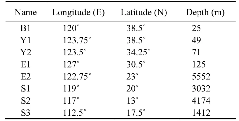
Table 1 Details of eight representative points

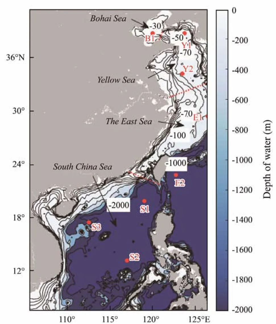
Fig.1 Topographic bathymetric map of the study area and eight representative points. The red dotted line represents the dividing line between different seas.

2.3 Methods

Extreme value theory is commonly adopted to analyze hydrometeorological extremes and their return levels and is also used for risk evaluation and management (Katzet al., 2002; Vasiliadeset al., 2015). The frequency analysis can provide a theoretical distribution function for extreme values; therefore, the users can obtain accurate results for a selected design return period (Coles, 2001). The generalized extreme value (GEV) distribution has been commonly applied in nonstationary conditions (Benistonet al.,2007; Towleret al., 2010; Katz, 2013). The GEV contains the following three parameters: location (μ), scale (σ),and shape (ξ). The NEVA method presented by Chenget al.(2014) was adopted in this study and has been used widely in investigating extreme climatic events (Swarnaet al.,2018;Patraet al.,2020; Galiatsatouet al.,2021; Lee and Park,2022).

The cumulative distribution function of the GEV can be expressed as (Coles, 2001):

where different cases ofξrepresent varying distribution functions. For a nonstationary process, the parameters of the underlying distribution function are time-dependent (Cooley, 2009) and the properties of the distribution change over time (Meehlet al., 2000). In NEVA, considering nonstationarity, the position parameter is assumed to be a linear function of time (Eq. (2)) while maintaining the scale and shape parameters as constants:

wheretis the time,µ0is the location parameter at timet0,andµ1is the regression coefficient usually preferred by the linear or log-linear models in hydrology literature.

3 Result

3.1 Annual Mean Extreme Significant Wave Height

Previous articles defined extreme wave height as selecting a maximum value from the overall wave height data.However, this method may provide unreliable samples due to the influence of extreme weather, such as typhoons, on extreme values. To overcome this shortcoming, the average of the top 2％ significant wave height is taken as the extreme wave at the grid point (Menéndezet al., 2008).The least square method was used for the trend study to obtain the trend in each grid.

Fig.2a shows the average annual distribution of extreme wave height and the long-time trend. The average annual extreme significant wave height in the BOS and YES is approximately 3 m and can reach 4.5 m in the southern YES.The average annual extreme significant wave height in the south of the ECS around the Taiwan Strait and the northeastern part of the SCS is approximately 5 – 6 m. The distribution of average annual extreme waves is closely related to water depth and typhoons. As the most frequently affected area, the eastern part of Taiwan Island is the area with the largest annual mean extreme wave height.

Fig.2b reveals that the extreme wave height in most areas of the ECS demonstrates a rising trend, with an increasing rate of approximately 0.025 m yr−1. Most areas in the SCS also show a rising trend, with an increasing rate of approximately 0.01 m yr−1. Furthermore, most areas in the BOS and YES and the surrounding areas of Hainan Island show a decreasing trend. The reduction range is approximately −0.005 – −0.01 m yr−1.

The sum of the extreme wave heights of each grid is divided by the number of grids to obtain the mean extreme wave heights of the entire region, which reflects the intensity of the extreme waves in the study area. Fig.3 shows its long-term trend in the study area from 1979 to 2018.The value fluctuates between 3.2 and 3.9 m in the study area, and the overall trend is increasing, among which the value in 1987 – 1988 and 1980 – 1981 fluctuates.

Fig.3 Long-term trend of annual extreme wave height from 1979 to 2018.

3.2 Seasonal Mean Extreme Significant Wave Height

The seasonal average and trend distribution of extreme wave height based on its seasonal statistics in 40 years are shown in Figs.4 and 5, respectively. Fig.4 shows that the seasonal average extreme wave height in spring is smaller than that in other seasons, and the extreme wave height in most sea areas in spring is approximately 3.0 – 4.0 m. The maximum extreme wave height located on the west side of the Taiwan Strait is approximately 4.5 m. The extreme wave heights in the southeast of the ECS are more than 5 m in summer, and the area with a mean extreme significant wave height of over 5 m has the largest proportion among the four seas. In autumn, seasonal extreme significant waves are largest for most of the study areas, and the largest value in the study area is concentrated in the southern part of the ECS and the middle and northern part of the SCS. In winter, the extreme wave height in the entire study area is generally high, and the extreme significant wave height in most sea areas is approximately 4 – 4.5 m.

Fig.4 Mean distribution of extreme wave height in four seasons from 1979 to 2018.

The trend of extreme waves in different seasons is obtained by linear fitting. The seasonal trend distribution of seasonal extreme wave height from 1979 to 2018 shows a reduction in the BOS and YES with a decreasing rate of approximately −0.005 m yr−1in spring, an increment in the ECS with an increasing rate of approximately 0.035 m yr−1, and a rise in most areas of the SCS with an increasing rate of 0.02 m yr−1. In summer and autumn, most parts of the SCS showed a decreasing trend of approximately−0.02 m yr−1, while the east part of Taiwan Island demonstrated a rising trend of approximately 0.04 m yr−1. In autumn, the northeast part of Taiwan Island and the northeastern part of the SCS showed an increasing trend of approximately 0.03 m yr−1and other areas revealed a decreasing trend. During the winter, most of the research areas demonstrated an increasing trend, and the largest increase rate occurred in the southern part of the SCS, with a value over 0.02 m yr−1. Meanwhile, BOS showed a decreasing trend with a value of approximately 0.01 m yr−1.

This paper also analyzed the trend of extreme waves in four seasons in the entire study area during the past 40 years to reflect the seasonal difference in the long-term trend(Fig.6). Zhang (2020) indicated that typhoons occurred more frequently from 1965 to the early 1970s, from the late 1980s to the late 1990s, and from the middle to the late 2010s. The frequency of typhoons relatively decreased from the 1970s to the late 1980s and from the late 1990s to the early 2010s. The frequency of typhoons in the Northwest Pacific decreased significantly with the slowdown of global warming in the late 1990s. Extreme wave heights are mainly caused by typhoons; thus, the fluctuations in the frequency and intensity of typhoons lead to significant fluctuations in extreme wave heights.

Fig.6 shows the extensive fluctuation range of annual mean extreme wave height in spring, wherein the maximum value can reach 3.3 m, the mean extreme wave height ranges from 1.9 m to 3.4 m, and the overall wave height is small.The fluctuation is most observed to be in 1991 – 1992. In summer, the annual mean extreme wave height fluctuated,and the annual mean extreme wave height ranged from 1.6 m to 3.6 m. The value significantly fluctuated in 1987– 1988, 1997 – 1998, and 2015 – 2016. The annual mean extreme wave height in autumn and winter fluctuated between 3.0 and 4.4 m, with abrupt changes occurring in 1981 – 1984 and 1992 – 1993, and the maximum fluctuation reached approximately 1.3 m in 1982 – 1993 in autumn.The annual mean extreme wave intensity of the entire area showed an increasing trend in spring and winter, demonstrating values of 0.99 and 0.66 cm yr−1, respectively. However, this intensity showed a decreasing trend in summer and autumn, revealing values of −0.03 and −0.02 cm yr−1,respectively. The conclusion obtained is consistent with that in Fig.5; that is, the order of increase or decrease rate is different due to the various statistical methods. However,they both proved the extreme wave height has fluctuating.

Fig.6 Seasonal distribution of extreme wave height trend from 1979 to 2018.

3.3 Extreme Significant Wave Height in Representative Points

The nonstationary method is adopted to analyze the variation characteristics of extreme waves in different seas, and the variation trend of extreme wave height with 50- and 100-year return levels is given.

1) Annual variation characteristics

Fig.7 shows the annual mean changes of extreme wave heights at different representative points. The figure indicates the variations in extreme wave changes in different representative points. Fig.7 also shows return levelsversusthe time covariate used in the linear regression (Eq. (2)).In this concept, the level of return changes over time; therefore, the probability of occurrence remains constant. For different representative points, the variation trend of wave height in the 50- and 100-year return periods is different.The interannual extreme wave in B1, Y1, and Y2 points slightly varies; therefore, the 50- and 100-year wave heights will not substantially change in the coming decades. The interannual extreme wave in E1, E2, S1, and S2 points shows an increasing trend, which indicates that the value of 50- and 100-year wave heights will rise in the next decades under the same risk. By contrast, the value will decrease in S3. This conclusion is crucial for ocean engineering, which determines the capability of ocean engineering to withstand extreme wave risk under the impact of climate change.

Fig.7 Effective return level of each point under the nonstationary hypothesis.

Figs.8 – 11 show the seasonal mean changes of extreme wave heights at different representative points. The figure reveals that the variation trend of the return period in different seasons is different. B1 and Y1 show a decreasing trend for spring; thus, the risk of extreme waves in these regions will be reduced under climate change. An increasing trend appears for other points, especially in E1 and S3,with rates of 0.02 and 0.016 m yr−1, respectively (Fig.8).

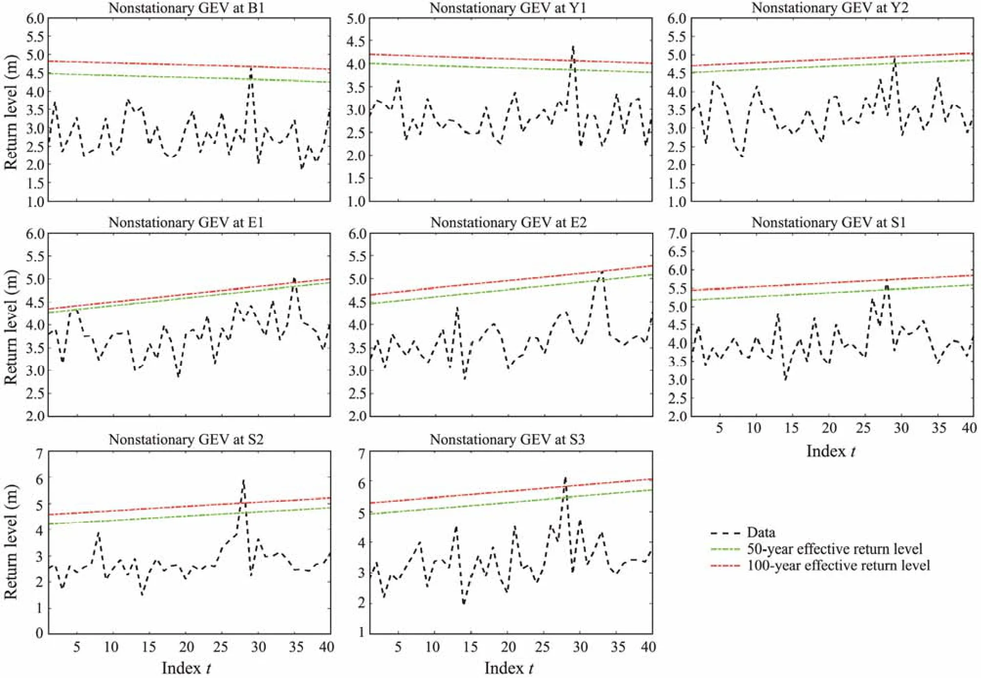
Fig.8 Effective return level of each point under the nonstationary hypothesis in spring.

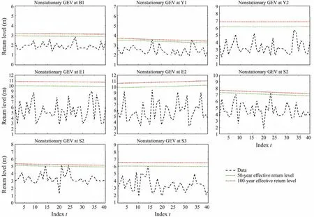
Fig.9 Effective return level of each point under the nonstationary hypothesis in summer.

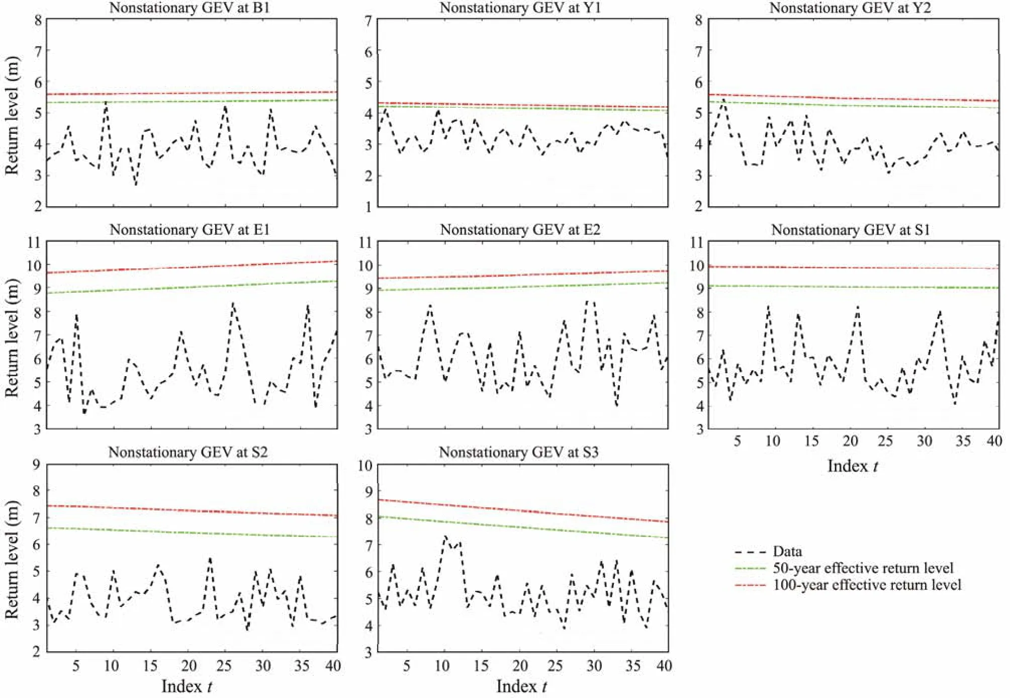
Fig.10 Effective return level of each point under the nonstationary hypothesis in autumn.

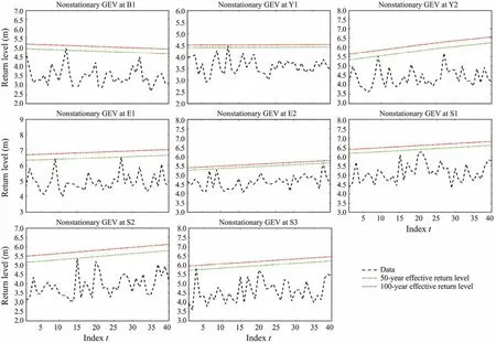
Fig.11 Effective return level of each point under the nonstationary hypothesis in winter.

2) Seasonal variation characteristics

The trends of 50- and 100-year wave heights in Y2 and S3 are not observed for summer. Therefore, extreme wave hazards in summer remain consistent with the current. The 50- and 100-year wave heights in E2 show an increasing tendency, demonstrating a rate of 0.01 m yr−1, which indicates the increasing risk of extreme wave height. A decreasing trend appears for other points, especially in S1,with a rate of 0.013 m yr−1.

For autumn, the trends of 50- and 100-year wave heights in B1 and S1 are not observed. Therefore, extreme wave hazards in summer remain consistent with the current. The 50- and 100-year wave heights in E1 and E2 show an increasing tendency, with the rate of 0.013 and 0.008 m yr−1,respectively, resulting in increased risks of extreme wave heights. The result is consistent with previous research,which indicates that typhoons will increase in intensity and move northward in the future (Mei and Xie, 2016). For the sea adjacent to China, most typhoons occur in the area where E1 and E2 are located, thus most frequently occurring in autumn. Other points show a decreasing trend,especially in S2 and S3, with the rate of 0.009 and 0.021 m yr−1, respectively.

For winter, the trend of 50- and 100-year wave heights in Y1 is also absent. Therefore, extreme wave hazards in summer remain consistent with the current. The 50- and 100-year wave heights in B1 show a decreasing trend with a rate of 0.007 m yr−1. The other points demonstrate increasing trends in winter, especially in Y2, with a rate of 0.024 m yr−1.

4 Discussion

The present results show that the distribution and trend of extreme waves are interannual and seasonal. The maximum extreme wave height in the study area is concentrated in the water northeast of Taiwan Island. The maximum seasonal mean extreme wave height appears in summer and autumn, and the minimum appears in spring. The results of linear fitting for the entire grids and the nonstationary analysis for eight points show varying trends of extreme waves at each point. The waters in the northeast of Taiwan Island show an increasing trend, while the other sea areas reveal different trends in various seasons. This study is the first to analyze trends for extreme waves over the past decades in the sea adjacent to China. Some scholars have also conducted some studies. Takbash and Young(2020) showed small reductions inin the Northern Hemisphere. For the water adjacent to China, Fig.4 of their paper revealed that the 100-year extreme waves show an increasing trend in the east and northeast of Taiwan Island,with a rising value of approximately 3 cm yr−1. However,the data were inadequate for most of the other waters in China. Thus, the influence of 100-year extreme waves during the 40 years remained unknown. Patraet al.(2020)showed that El Niño induced large extreme waves over the western North Pacific during summer and autumn. Osinowoet al.(2016) showed that trends larger than 0.05 m yr−1were distributed over a large part of the central SCS.In this article, the authors defined extreme waves as 99th percentile significant wave height. Except for autumn, the extreme waves in the three other seasons showed an increasing trend. Liet al.(2020) demonstrated consistently increasing extreme wave heights throughout northern ECS.

Hence, all these findings are consistent with the present results. However, the present study compensates for the shortcomings of previous studies. For example, Liet al.(2020) only focused on ECS, and the nonstationary method was not adopted. Younget al.(2012) only included part of the sea area, and most areas did not pass the significance test. The average of the top 2％ wave height of each grid point is defined in the current paper as the extreme wave height, which avoids the randomness caused by typhoons and provides practical research results. The characteristics of seasonal changes for extreme waves are also examined in the present study.

5 Conclusions

The present study analyzed the temporal and spatial distribution characteristics of extreme waves in the water adjacent to China. A nonstationary analysis method is also adopted in eight points to investigate the trend of 50- and 100-year wave heights. The result is consistent with previous results.

The results reveal that the mean value of extreme waves is the largest in the eastern part of Taiwan Island and the smallest in BOS from 1979 to 2018. In the study area,only the extreme wave height in the northeastern part of Taiwan Island shows a significant increasing trend. For most of the SCS, the extreme wave heights in summer and autumn show a decreasing trend, which is related to the northward movement of the typhoon track and the decreasing trend of typhoon intensity.

Nonstationary analysis shows considerable variations in the values of 50- and 100-year significant wave heights in eight points. Considering the annual mean change, E1,E2, S1, and S2 present an increasing trend, and S3 shows a decreasing trend. For the seasonal mean change, most points reveal an increasing trend in spring and winter,while others show a decreasing trend in summer and autumn. Notably, the E1 point growth rate is large in autumn,which is related to the change in typhoon intensity and the northward movement of the typhoon path.

At present, many scholars have studied the weather change process under different greenhouse gas emission backgrounds (Bernardinoet al., 2021; Lemoset al., 2021)and also analyzed the characteristics of wave change. The research in this paper can be applied to the future study of extreme wave changes and the analysis of extreme wave risks under different greenhouse gas emission backgrounds.

Acknowledgements

The authors gratefully acknowledge the support of the Natural Science Foundation of China (No. 51909114), and the Major Research Grant (Nos. U1806227, U1906231) from the National Natural Science Foundation of China (NSFC).