The Variation of Plankton Community Structure in Artificial Reef Area and Adjacent Waters in Haizhou Bay

GAO Shike , SHI Yixi , LU Yanan and ZHANG Shuo

1) College of Marine Sciences, Shanghai Ocean University, Shanghai 201306, China

2) Joint Laboratory for Monitoring and Conservation of Aquatic Living Resources in the Yangtze Estuary,Shanghai 200000, China

Abstract Plankton are an important component of marine protected areas (MPAs), and its communities would require much smaller interpatch distances to ensure connection among MPAs. According to the survey from MPAs dominated by artificial reefs and adjacent waters (estuary area (EA), aquaculture area (AA), artificial reef area (ARA), natural area (NA) and comprehensive effect area (CEA)) in Haizhou Bay in spring and autumn, we analyzed phyto-zooplankton composition, abundance and biomass, and correlation with hydrologic variables to gain information about the forces that structure the plankton. The results showed that the dominant zooplankton were copepods (spring, 98.9％; autumn, 94.2％), while the phytoplankton were mainly composed of Bacillariophyta (spring, 61.8％; autumn, 95.6％). The RDA results showed that temperature, salinity and depth highly associated with the distribution and composition of plankton species among the habitats than other factors in spring; temperature, Chla and DO had the strongest influence in autumn. The zooplankton in the ARA and AA ecosystems basically contained the same species as those in other habitats, and each habitat also exhibited a relatively unique combination of plankton species. The structures of the EA zooplankton in spring and the EA phytoplankton in both seasons were much different than other habitats, which may have been caused by factors such as currents and tides. We concluded that there exists similarity of the plankton community between artificial reef area and adjacent waters, whereas the EAs may be relatively independent systems. Therefore, these interaction between plankton community should be considered when designing MPA networks, and ocean circulations should be considered more than the environmental factors.

Key words zooplankton; phytoplankton; seasonal variation; environmental factor; artificial reef

1 Introduction

Marine protected areas (MPAs) dominated by artificial habitats are known to enhance the abundance and diversity of species and have been shown to contribute to restoration and habitat recovery in marine environments;thus, MPAs are increasingly envisaged as tools for managing coastal ecosystems and fisheries. (Clark and Edwards 1999; Galzinet al., 2006; Anadónet al., 2013;Folppet al., 2020). To address the large-scale conservation challenges facing coastal marine ecosystems, several nations are building MPAs and MPA networks, and the marine habitats and fisheries supported by these MPAs may be modified through the use of artificial habitats placed in the sea (Moraet al., 2006; Planeset al., 2009;Gaineset al., 2010).

Haizhou Bay is a medium-sized offshore area covered by a shallow temperate continental shelf; this bay is mainly affected by a branch of the Yellow Sea Warm Current and the coastal currents that flow from northeast to southwest (Sunet al., 2003; Zhanget al., 2017). Since 2002, the local government has begun to build MPAs dominated by artificial reefs aiming at ecological restoration and resource conservation to support the planning and management of marine resources in Haizhou Bay(Zhanget al., 2006; Wuet al., 2012). These MPAs support an area in Haizhou Bay with a high conservation value, containing various habitats (estuaries, tidal mudflats, artificial reef area and mariculture areas (Wuet al.,2012; Zhaoet al., 2015). However, the relationships among these habitats have not yet been fully studied.

Plankton are an important component of aquatic ecosystems; phytoplankton are one of the primary producers of aquatic environments, and zooplankton are a key link in the food web (Douet al., 2016; Xiaoet al., 2020);plankton diversity is mainly determined by the dispersal of propagules along ocean currents (Goetze, 2005; Villarinoet al., 2018). In offshore marine environments, the placement of artificial habitats changes the local flow patterns, producing upwelling and eddy currents and causing the bottom-up movement of nutrients, thus promoting the growth and reproduction of plankton and ultimately influencing fishery resources (Yanget al., 2012;Championet al., 2015; Wanget al., 2019). Differences in plankton abundance among taxa are thought to play a major role in determining the distribution pattern and scale of marine plankton dispersal (Finlayet al., 2002;Villarinoet al., 2018). To understand how marine biodiversity is locally and spatially maintained, it is necessary to study the relationship between plankton dispersal and local abundance. In addition, sharp environmental factors and other oceanographic features represent barriers to plankton dispersal; for example, changes in the water environment, including the temperature, salinity, dissolved oxygen, pH, nutrient concentrations, or phytoplankton and fish biomass, can directly or indirectly affect the abundance, distribution and community structure of plankton (Yebraet al., 2011; Yanget al., 2012). Thus,it may be possible to restore plankton diversity by modulating environmental factors and to improve the structure and function of ecosystems by exploiting the plankton communities (Mckinnonet al., 2015; Daiet al., 2019;Xiaoet al., 2020).

Most studies have considered only fish species and have not included other taxonomic groups, such as plankton; these other groups would presumably require much smaller interpatch distances to ensure connection among MPAs (López-Sanzet al., 2009; Folppet al., 2013;Guinderet al., 2020). In this study, 1) the phyto-zooplankton abundance and its relationships to environmental factors in artificial reef area and adjacent waters were compared to explore the links between habitats; 2) the similarity and difference of these plankton were analyzed to explore the plankton distribution pattern among habitats and seasons. Our results will have a significant reference value in terms of the links in small patches of the food web basis and better understanding in deeply designing MPA networks in Haihzou Bay.

2 Materials and Methods

2.1 Study Area

Haizhou Bay, located west of the coast of Lianyungang City, Jiangsu Province, north of the Qingdao Fishing Ground, and south of the Lvsi Fishing Ground, is mainly composed of sandy and muddy habitats and represents an open bay with an area of approximately 877 km2(Wang,1993). The climate and hydrology of Haizhou Bay are greatly influenced by the mainland, and most fishing areas in this region are controlled by coastal currents (Sunet al., 2003; Zhanget al., 2017). Under the influence of the Yellow Sea Coastal Current (YSCC) and the Yellow Sea Warm Current (YSWC) (Fig.1), the flows merge to form a rotating flow in the estuary of Haizhou Bay (Xieet al., 2007). Therefore, according to the geographic information system, we divided the survey area into five areas (Table 1). The investigations were conducted in October 19 – 23, 2020 (autumn) and April 26 – 29, 2021(spring), in which the fishery resources and water environment were at the best status, and 24 site locations were obser- ved (Fig.1). Environmental data were collected by a single ship (Su Ganyu Yang 01388) at each site, with depth range between 6.54 – 12.56 m.

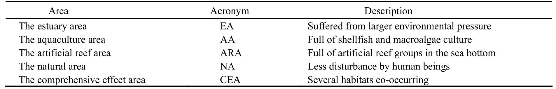
Table 1 The description of the divided area in Haizhou Bay

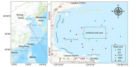
Fig.1 Study area and sampling sites.

The acronym and description of each habitat are listed in Table 1. The same notation is used in the figures below.The black rectangle box is artificial reef area. YSWC is the Yellow Sea Warm Current, YSCC is the Yellow Sea Coastal Current and ECSCC is the East China Sea Coastal Current.

2.2 Sample Collection

Salinity, temperature, and depth at vertical direction(surface to bottom water) were recorded by a CTD (RBR concerto, Canada) measuring system. pH and dissolved oxygen (DO) were measured with a SMART pH meter(pH-818) and a SMART SENSOR dissolved oxygen meter (AR8210) respectively. The surface water samples were collected by an organic glass hydrophore. A total of 2 L of water samples (1 L for nutrients and 1 L for chlorophylla(Chla)) were stored in a polyethylene bottle and brought back to the laboratory for water chemical variables analysis. The several dozen grams of sediment samples were collected by a bottom sampler at the same times.The shallow water plankton net (37 cm in diameter, mesh 0.077 mm for phytoplankton, and 50 cm in diameter, mesh 0.505 mm for zooplankton) is filtered vertically from the seafloor to the surface by winch with speed of 0.5 m s−1.The filtrate was placed in the polyethylene bottle (1 L for zooplankton and phytoplankton respectively) and immediately added with 90％ formaldehyde-solution to kill the zooplankton and other organisms.

The water, sediments and plankton samples were collected at each site, and preserved and analyzed in accordance with the national standard of the People’s Republic of China ‘Code for Marine Survey’ (GB12763-2007).

2.3 Chemical Analysis

Nitrate nitrogen (NO3−-N), nitrite nitrogen (NO2−-N),silicate (SiO32−-Si), active phosphate (PO43−-P) and ammonia nitrogen (NH4+-N) and the concentration of Chlain the water samples were determined by spectrophotometry method (UV-1200). Total nitrogen (TN) and total phosphorus (TP) in the sediment samples were analyzed using DigiPREP TKN Systems (KDN-1) and spectrophotometry method (UV-1200), respectively.

2.4 Plankton Determination

For determination of zooplankton, samples were taken back to the laboratory to identify to species level with stereoscopic microscopy (OLYMPUS BX35 and OLYM PUS SZX16). The number of zooplankton was obtained by microscopic counting, and their biomass was determined using the volumetric method (Yinet al., 2018). For phytoplankton, the supernatant was removed and left with about 20 – 30 mL after the water samples were precipitated for 48 h (Larssonet al., 2017). A total of 0.1 mL of the well-shaken concentrated sample was put in a 0.1 mL phytoplankton count chambers, and then the phytoplankton were identified and counted with a microscopy(OLYMPUS BX35, field lens 40 × eye lens 10) to obtain the numbers of phytoplankton per unit volume (1 L). The methods to quantify volume and biomass of zooplankton were the same as those to phytoplankton.

2.5 Statistical Analyses

2.5.1 Alpha diversity

The dominance degree (Y), Shannon index (H’) and Simpson index (D) were mainly used to analyze alpha diversity of plankton (Lindley and Batten, 2002). The calculation formula is as follows:

where,niis the number of individuals of theith species,Nis the total number of individuals, andPiis the ratio of the number of individuals (ni) of theith species to the total number of individuals (N) (ni/N). The species with a dominance degree greater than 0.02 were selected as the dominant species.

2.5.2 Beta diversity

All data conform to normal distribution according to the normal distribution and homogeneity tests. Analysis of variance (ANOVA) applied to the log-transformed zooplankton abundance data with the critical probability level set at 0.05 was used to analyze the difference between environmental factors. Based on Bray-Curtis similarity,the results were visualized by nonmetric multidimensional scale analysis (NMDS) to evaluate the distribution of species in different habitats. Nonparametric multivariate analysis of variance (PERMANOVA; α = 0.05) was used to analyze the differences in phyto-zooplankton community between habitats. The count data were Hellinger-transformed (Legendre and Gallagher, 2001) and subjected to Redundancy Analysis (RDA) (Rao, 1964;Jongmanet al., 1995), which allowed the relationships between samples and between taxa to be visualized.

2.5.3 Data analysis

Arcgis software (v. 10.7) was used to draw survey map.PERMANOVA, NMDS and RDA were conducted with the Vegan package within R (v.4.1.2) (R Development Core Team, 2009). All data were pretreated and performed in Excel 2021.

3 Results

3.1 Study Area Description

The main environmental factors among habitats are shown in Fig.2. In both spring and autumn, the minimum value of depth, temperature and salinity were both occurred in EA. In autumn, the DO and Chlacontents decreased from the AA to NA; the maximum contents of both DO and Chlaoccurred in the AA (8.60 mg L−1and 8.92 μg L−1, respectively), and no significant variation occurred in spring. In the two seasons, the NO3−, NO2−,SiO32−and NH4+contents had a gradual decreasing trend among from EA to NA, while the PO43−content showed an opposite trend in autumn. The TP and TN contents showed decreasing trends in autumn, but a different trend in spring.

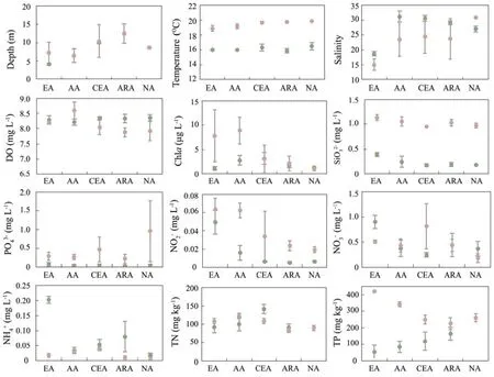
Fig.2 Physicochemical parameters of the water samples obtained from different habitats in Haizhou Bay. The green dots represent spring, and the brown dots represent autumn.

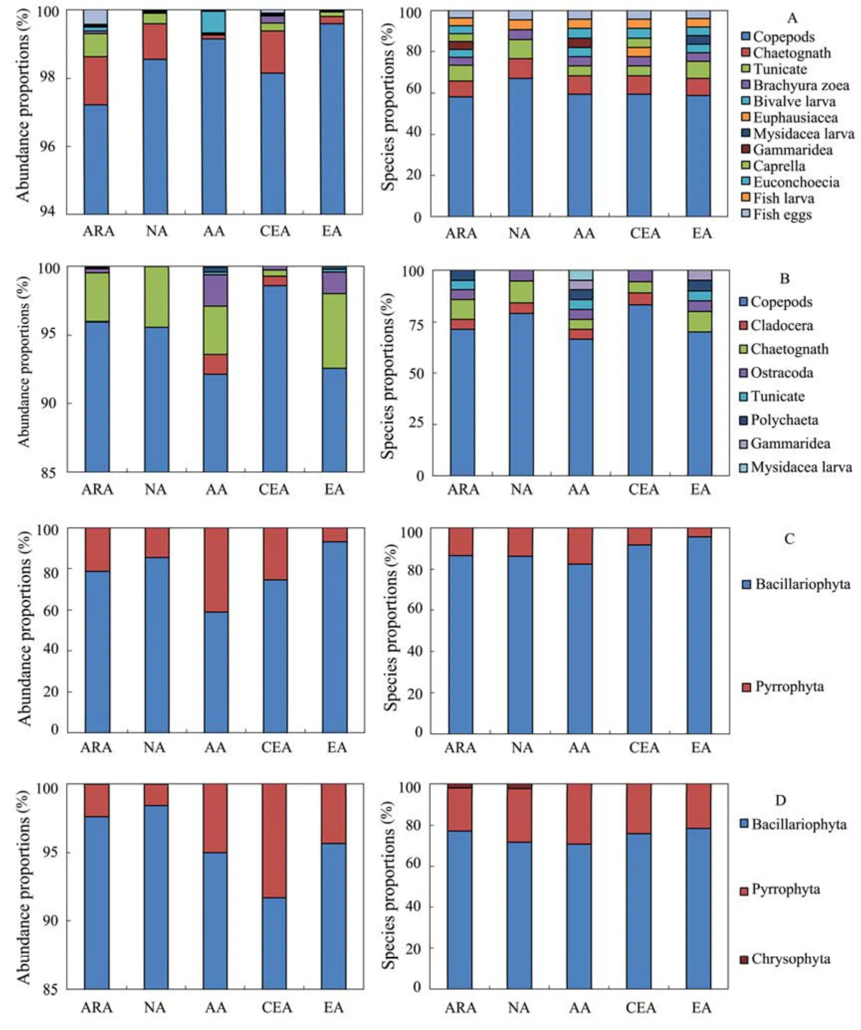
Fig.3 Zooplankton and phytoplankton individuals and species identified in the five habitats. A, spring zooplankton; B, autumn zooplankton; C, spring phytoplankton; D, autumn phytoplankton.

3.2 Plankton Community Composition

In spring, a total of 32 zooplankton species and 52 phytoplankton species were observed; In autumn, a total of 29 zooplankton species and 65 phytoplankton species were observed. Most of the zooplankton were copepods,accounting for 98.9％ and 94.2％ of the overall zooplankton abundance in spring and autumn, respectively (Figs.3A, B); the phytoplankton were mainly composed of Bacillariophyta, accounting for 61.8％ and 95.6％ in spring and autumn, respectively (Figs.3C, D).

The dominant (Y> 0.02) zooplankton and phytoplankton species are shown in Table 2. In spring,Acartia bifilosa, a copepod, had the highest dominance among the zooplankton species, with a dominance of 0.86, whileCalanus sinicus, another copepod, was the most dominant species in autumn, with aYvalue of 0.29. Among the phytoplankton,Nitzschia paradoxa(Y= 0.22), which belongs to Bacillariophyta, were the relatively dominant species in spring, andThalassionema frauenfeldii(Y=0.49) of Bacillariophyta was the dominant species in autumn.

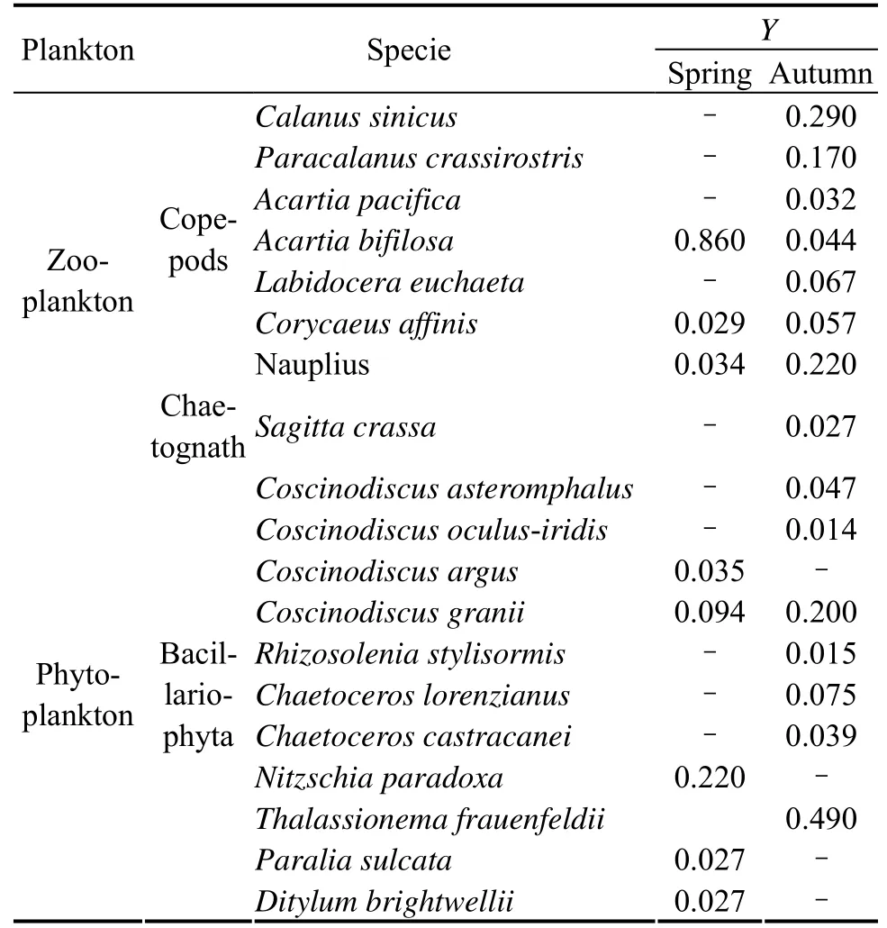
Table 2 Dominant zooplankton and phytoplankton species

3.3 Alpha Diversity of Plankton

The plankton abundance and diversity values calculated from the samples are shown in Fig.4. The zooplankton abundance was highest in the AA (spring: 222820 ±36644 ind. m−3; autumn: 4496 ± 2814 ind. m−3) in both seasons, while that in the NA was the lowest (366 ± 231 ind.m−3) in autumn; the highest phytoplankton abundance was found in the EA, with an average value of 3.7 × 107ind. m−3in autumn. The variations in the Shannon index values of zooplankton and phytoplankton showed the same trends as the corresponding Simpson index values.In spring, the highest Shannon index and Simpson index values for zooplankton were found in the CEA, and the lowest values were found in the AA; in autumn, the highest values were found in the CEA, and the lowest were found in the EA. However, when ordered using the Shannon index and Simpson index values determined for phytoplankton, the habitats were ranked as NA, ARA, EA,CEA and AA from high to low in autumn and as AA,ARA, EA, CEA, and NA, from high to low, in spring.Generally, the Shannon index and Simpson index values determined for zooplankton were higher in autumn than in spring, while the opposite trends were observed for phytoplankton in both seasons.

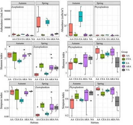
Fig.4 The abundance, Shannon and Simpson index of zooplankton and phytoplankton between the five habitats.

3.4 Beta Diversity of Plankton

Combined with univariate PERMANOVA, the clustering results were visualized using NMDS (Fig.5). The zooplankton abundances determined in the five habitats differed significantly between the two seasons (P= 0.004 and 0.001,n= 5) (Table 3). There were significant differences phytoplankton abundance among all the habitats in spring (P= 0.001,n= 5), but no significant differences in autumn (P= 0.089,n= 5) (Table 4). A posteriori analysis showed that significant differences were observed in zooplankton abundance between ARA/AA, ARA/EA, CEA/AA and NA/AA in spring (P< 0.05) (Fig.5A). In autumn,significant differences were only observed in ARA/EA and NA/AA (P≤ 0.05) (Fig.5B). For phytoplankton, significant differences were found in ARA/AA, ARA/EA,CEA/AA and NA/AA in spring (P≤ 0.05) (Fig.5C), but no significant differences were found between any habitats in autumn (Fig.5D). Generally, the structure of phytoplankton community showed a larger seasonal variation than the zooplankton did.

Table 3 Univariate PERMANOVA results obtained for the overall and pound-by-pair zooplankton species abundance interactions in the five habitats

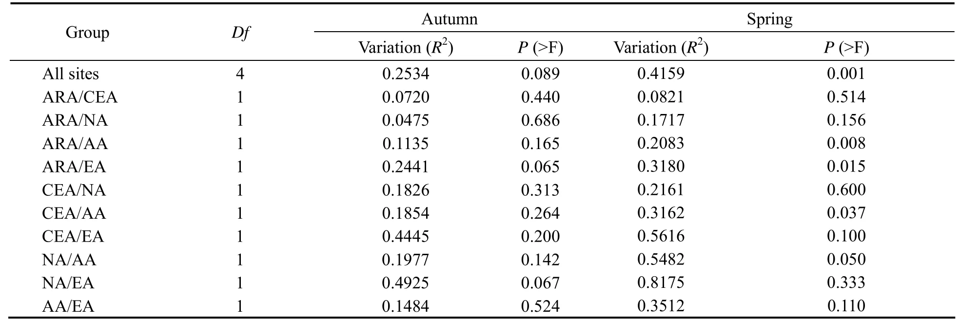
Table 4 Univariate PERMANOVA results for the overall and pound-by-pair phytoplankton species abundance interactions in the five habitats

Fig.5 Visualization of the NMDS results for the plankton abundance measured in samples obtained from different habitats.The different colored points represent the different habitat types, and each point indicates a sampling site. A, Spring zooplankton; B, autumn zooplankton; C, spring phytoplankton; D, autumn phytoplankton.

Different habitat types and plankton taxa with similar habitat associations in both seasons could be identified in Fig.6. We can intuitively see that each habitat contains specific species in each season, and these species distributions reflect strong positive correlations among habitats.Additionally, the same species can also be found in different habitats simultaneously (e.g., some zooplankton are shared among the EA, ARA and AA in autumn, and some phytoplankton are identified in both the AA and EA in autumn), implying the potential association of plankton community among habitats.

3.5 Relationships Between Plankton Community and Environmental Factors

The RDA results are shown in Fig.7. For zooplankton,the first two axes contributed 11.2％ of the variance in the zooplankton species data and 3.7％ of the species-environment relations in spring; these values were 6.9％ and 3.0％, respectively, in autumn. For phytoplankton, the first two axes contributed 10.4％ of the variance in phytoplankton species data and 35.6％ of the species-environment relations in spring, with corresponding values of 9.0％ and 9.1％, respectively, in autumn. The RDA results of the plankton abundance and environmental factors showed that the depth, temperature, salinity, DO, Chla,TN, TP and nutrients were the main factors affecting the abundance of plankton. For zooplankton, in spring, no species showed any positive correlation with the environmental factors; in autumn, most Polychaeta and Ostracoda species abundances were positively correlated with NH4+, TN and TP, and most copepod and chaetognath species abundances were positively correlated with DO. For phytoplankton, in spring, most Pyrrophyta species were quite positively correlated with Chlaand salinity, while in autumn, most Pyrrophyta species were positively correlated with DO. Overall, salinity and depth had the strongest influence on the distribution and composition of plankton species in spring, while temperature,Chla and DO had the strongest influence in autumn.

Fig.7 RDA results obtained between environmental factors and plankton species. The colored points represent the plankton abundances obtained in different habitat types. The smaller black points represent the plankton species, and the arrows represent environmental factors. A, spring zooplankton; B, autumn zooplankton; C, spring phytoplankton; D, autumn phytoplankton.

4 Discussion

4.1 Plankton Community and Its Relationship with Environmental Factors

In this study, copepods and diatoms occupied the majority of zooplankton and phytoplankton all the habitats,which were consistent with previous surveys in Haizhou Bay and the Yellow Sea (Wanget al., 2011; Yanget al.,2012; Xieet al., 2017; Zhanget al., 2017; Wanget al.,2019). The largest numbers of zooplankton individuals and species and the highest zooplankton abundances appeared in the AA in both seasons, and this may have been due to the large numbers of benthic organisms and macroalgae cultured in the AA in Haizhou Bay; the faeces and residues of these organisms may prompt the proliferation of phytoplankton, thus directly providing sufficient dietary sustenance for zooplankton (Suet al., 2019). The ARA had the highest numbers of plankton species among all habitats in both seasons, and the abundance and diversity index values were maintained at relatively low levels.On the one hand, the construction of artificial reefs is conducive to increasing plankton biomass and abundance,leading to an increased zooplankton diversity (Chenet al.,2014; Daiet al., 2018); on the other hand, the main factors affecting the abundance and species distribution of plankton include not only ocean currents and water environments but also predator-prey dynamics (Augeret al.,2014; Mckinnonet al., 2015; Gretchenet al., 2020; Xiaoet al., 2020). Geographically, the ARA contains relatively rich fishery resources and is located close to the NA,where fish, shrimp, and other aquatic organisms require large intakes of plankton for their growth and development (Xieet al., 2017; Zhanget al., 2017; Daiet al.,2019). The results also revealed that in the EA, there were high levels of zooplankton abundance in spring and phytoplankton abundance in autumn, but the zooplankton diversity index was the lowest in this habitat, and no significant difference was found in the phytoplankton diversity index (Fig.4). Estuaries are regarded as important transitional zones where nutrients sourced from the land and sea mix to produce highly spatially heterogenous conditions (Pasquaudet al., 2008; Howeet al., 2017).The tributaries of the Yellow Sea Warm Current form a southwest-northeast circumfluence at the estuary area of Haizhou Bay, which make a seasonal variation in this region, resulting in higher primary productivity in spring(Sunet al., 2003; Zhanget al., 2017). In addition, a low concentration of diatoms, the main food source of copepods, also inhibits the reproduction, growth and development of copepods. The zooplankton and phytoplankton abundances decreased from the EA to the NA in both seasons, and this result was consistent with the rule that more species were identified in the offshore phytoplankton communities than in the coastal marine phytoplankton communities (Xiaoet al., 2020).

Changes in the compositions and quantitative structures of plankton communities are mutually restricted by various environmental factors. In this study, salinity and depth were the most important environmental factors affecting the community structure of plankton in spring.Due to the complex hydrological conditions in the South Yellow Sea, the salinity structures differ greatly among different habitats, and different zooplankton species respond differently to different environmental conditions(Ronget al., 2003; Liet al., 2004). In our results, the salinity variation was much larger to plankton among habitats in both seasons (Fig.6), further verifying this finding.Depth is another factor affecting the plankton distribution.Tosettoet al. (2021) believed that some species of planktonic cnidarian, which were abundant in all sampled neritic sites, were positively related to higher shallow depths (< 70 m). The study of Liet al. (2015) showed that the ichthyoplankton abundance was positively correlated with depth (20 – 40 m) in Haizhou Bay. Unfortunately, we did not collect plankton samples along vertical factors in this survey; this sampling scheme will be supplemented in subsequent surveys. Previous studies have shown that the diurnal vertical migration of zooplankton is closely linked to changes in the water temperature (Granataet al.,2020). Moreover, the feeding behaviour of zooplankton cause the Chlaconcentration to decrease. When the zooplankton biomass increases, the oxygen consumption rate also increases, resulting in a decreased DO concentration(Calbetet al., 2005; Iriarteet al., 2012; Granataet al.,2020). This process could explain why the temperature,Chlaand DO represent the most important environmental factors in autumn. Among nutrients, PO43−, NO3−and SiO32−were identified as important biogenic elements for phytoplankton, and decreases in the concentrations of these nutrients lead to changes in the abundance and distribution of phytoplankton, thus indirectly affecting the growth and development of zooplankton and even changing the entire structure of the surficial marine food web(Caricet al., 2012; Iriarteet al., 2012; Bharathiet al.,2018). While Fig.6 also intuitively shows that nutrients were slightly more correlated with the phytoplankton abundances among species but not among habitats. This may imply that nutrients were not the main factors influencing the plankton community abundance variations among habitats. Generally, we believe that the temperature, salinity, Chla, DO and depth were the main environmental factors driving the observed changes in the plankton community structure among habitats in the two studied seasons.

4.2 Plankton Distribution Pattern Between Artificial Reef Area and Adjacent Waters

Ocean currents are a decisive force in the construction of plankton communities in marine ecosystems (Watsonet al., 2011; Tosettoet al., 2021). A high level of species similarity leads to and similar compositions, abundance,diversity, and biomass variation patterns (Granado and Henry, 2014). Basically, the zooplankton communities in the ARA/AA were different, but some same species occurred in other habitats, possibly indicating potential links between the ARA and the AA with other habitats, further supporting the positive effects induced by the successful construction of artificial reefs in Haizhou Bay increasing the plankton species abundance. Moreover, each habitat also exhibited a relatively unique combination of plankton species in each season. The dispersal and settlement processes of organisms may lead to the natural aggregation of habitats that were originally spatially discrete(Karen, 2014), suggesting the existence of some underlying associations between previously noncontiguous habitats. Certainly, we cannot make a generalization using only one standard because some environmental factors and predators may also contribute to differences in plankton community structures among different harbour regions. However, surface current transport times have been found to be more important than environmental factors in explaining spatial changes in plankton community similarity (Villarinoet al., 2018). According to our results,other than the temperature, salinity, Chla, DO and depth,environmental factors greatly influenced only the plankton species compositions and could not effectively explain the community differences observed among habitats(Fig.7).

The EA in Haizhou Bay is a major source of discharge to the ocean, and has an average annual runoff of 1.7 billion m3(Fuet al., 2017). The structure of the zooplankton community in the EA in spring and that of the phytoplankton community in the EA in autumn were much different from those in other habitats (Fig.5). This may have been caused by factors such as ocean currents and tides. The coastal circumfluence formed by the continental coastal current and the Yellow Sea Warm Current may also block and recombine the zooplankton community structure, and the water level in the EA fluctuates due to the intermittent influence of tides, leading to the formation of meta-communities (linked local communities connected by dispersal) (Leiboldet al., 2004; Reiset al.,2019). Some evidence has shown that circulation dynamics and the intermittent influence of tides in EAs have the potential to drive variations in the distribution and abundance of zooplankton communities (Daiet al., 2016; Reiset al., 2019), making it difficult to form links between EAs and adjacent habitats. After all, many estuaries in different regions are characterized by the dynamic interplay among physical, chemical, geological and biological processes, including some other biotic (e.g., inter- and intra specific competition) and abiotic (e.g., season variations) factors that affect plankton abundances and communities (Robinset al., 2016; Gretchenet al., 2020); this topic remains a complex and comprehensive challenge that will be addressed in future research.

5 Conclusions

In this study, we concluded that there exists similarity of plankton community between artificial reef area and adjacent waters in Haizhou Bay, while the EA may be a relatively independent system. Moreover, nutrients may have an influence on some plankton species, and the temperature, salinity, Chla, DO and depth had the strongest driving influence to the plankton community structures among habitats seasonally; however, these factors cannot effectively explain the plankton community differences observed among habitats. Therefore, we suggest that MPAs or MPA networks should be designed with greater consideration of plankton community interaction and seasonal variation between adjacent habitats and that ocean circulations such as tidal currents and upwellings should be considered more than environmental factors.

Acknowledgements

This study was financed by the Jiangsu Haizhou Bay National Sea Ranching Demonstration Project (No. D-80 05-18-0188), and the Shanghai Municipal Science and Technology Commission Local Capacity Construction Project (No. 21010502200).