Slowing down of the summer Southern Hemisphere Annular Mode trend against the background of ozone recovery
2024-03-04FeiZheng
Fei Zheng a , b , ∗
a School of Atmospheric Sciences, Key Laboratory of Tropical Atmosphere-Ocean System, Ministry of Education, Sun Yat-sen University, Zhuhai, China
b Southern Marine Science and Engineering Guangdong Laboratory, Zhuhai, China
Keywords:
ABSTRACT Observations show significant trends in Southern Hemisphere extratropical climate in the late 20th century,including a strong positive trend in the austral summer Southern Hemisphere Annular Mode (SAM) accompanied by warming of the Antarctic Peninsula and melting sea ice in the Bellingshausen Sea.Statistical analysis and model simulations have shown that these trends were driven mainly by Antarctic stratospheric ozone depletion.Here,results show that the widely reported summer SAM trend has flattened since around the year 2001 against the background of the ozone recovery, supporting results from previous model simulations that predicted a slowing down of the well-documented positive summer SAM trend.Four SAM indices based on different definitions from different datasets show consistency in this slowdown.Furthermore, changes in surface air temperature (SAT) in the Antarctic and sea-ice concentration (SIC) around the Antarctic are detected.Different from the SAM, in which the signs of trends only slow down but do not reverse after the ozone recovery, the signs of trends in Antarctic SAT and SIC have reversed.The warming of the Antarctic Peninsula has turned into a cooling trend, and the melting of sea ice in the Bellingshausen Sea has turned into an increasing trend.Additional diagnostics studies with observational and model data could go a long way towards enhancing our understanding of changes in Southern Hemisphere surface climate against the background of ozone recovery.
1.Introduction
The dominant mode of atmospheric circulation in the Southern Hemisphere extratropics is well-known as the Southern Hemisphere Annular Mode (SAM), otherwise known as the Antarctic Oscillation,which is an intrinsic atmospheric mode and the dynamics involve eddy–zonal mean flow interactions ( Lorenz and Hartmann, 2001 ; Zhang et al.,2012 ).A positive phase of the SAM reflects low-pressure anomalies over high latitudes and high-pressure anomalies over the middle latitudes.The increasing pressure gradient in the positive SAM phase causes poleward movement of the westerly jet, and vice versa ( Gong and Wang, 1998 ; Thompson and Wallace, 2000 ; Li and Wang, 2003 ).The SAM impacts many aspects of Southern Hemisphere climate, including Antarctic surface temperatures, extratropical precipitation, and sea ice( Li and McGregor, 2017 ; Fogt et al., 2022 ).Evidence also shows that tropical climate and even Northern Hemisphere climate are related with the SAM ( Wang and Fan, 2005 ; Gong et al., 2009 ; Zheng et al., 2015 ;Dou and Wu, 2018 ).
The SAM experienced profound changes in the late 20th century( Thompson et al., 2011 ; Fogt and Marshall, 2020 ).A positive trend was observed in the SAM, which can be mainly attributed to Antarctic stratospheric ozone depletion, with the increasing CO2also playing a role( Gillett and Thompson, 2003 ; Arblaster and Meehl, 2006 ; Polvani et al.,2011a ).The responses of extratropical circulation to increasing CO2exhibit a similar pattern as those to Antarctic ozone depletion, including a strengthening of the polar vortex and a poleward shift of the polar jet, i.e., a positive SAM, but the positive SAM trend is mainly caused by ozone depletion ( Kushner et al., 2004 ; Arblaster and Meehl, 2006 ).Antarctic ozone depletion cools stratospheric air temperatures, resulting in stronger stratospheric westerly winds near 60°S.The anomalies in the stratosphere then transport downwards to the troposphere and lead to a positive SAM phase.The strongest ozone depletion occurs in austral spring, and thus the SAM trend also exhibits clear seasonality,with the strongest positive trend occurring in austral summer, lagging stratospheric ozone depletion by one season ( Thompson et al., 2011 ;Previdi and Polvani, 2014 ; Fogt and Marshall, 2020 ).
Through the 21st century, however, Antarctic stratospheric ozone is expected to recover thanks to the Montreal Protocol.The emergence of this healing of the Antarctic ozone layer has been observed( Kuttippurath et al., 2013 ; Solomon et al., 2016 ).Model simulations show that ozone recovery is likely to lead to a negative summer SAM( Son et al., 2008 ; Polvani et al., 2011b ), while increasing CO2is likely to result in a positive summer SAM, counteracting the effect of ozone recovery ( Arblaster et al., 2011 ; Polvani et al., 2011b ; McLandress et al.,2011 ).Given that ozone recovery and increasing CO2are expected to have opposing effects on the summer SAM, the well-documented positive trends are predicted by model simulations to be weakened.A negative SAM trend is also expected with the continuous recovery of Antarctic stratospheric ozone, but whether a reversing of the SAM trend will emerge, or when the opposing trend will occur, is a complex question.
Although model studies have as mentioned predicted a weakening SAM trend against the background of ozone recovery, less attention has been paid to detecting a decrease in the SAM trend in observations due to the limited length of data.However, now that 20 years have passed since the beginning of the ozone recovery in around 2001,it is possible to compare changes in the SAM trend during the ozone depletion and recovery periods.As a matter of fact, changes in stratospheric circulation have been detected in observations: the post-2001 trends of stratospheric temperature and circulation have shown significant changes with the pre-2001 trends, and the underlying reason is attributable to Antarctic stratospheric ozone recovery ( Banerjee et al.,2020 ; Zambri et al., 2021 ).
This paper focuses on the summer SAM, a major atmospheric circulation signal in the troposphere, and analyzes whether the weakening of the summer SAM trend has emerged in observations against the background of ozone recovery.Given that the extratropical surface climate is largely modulated by the SAM, the changes in summer Antarctic surface air temperature (SAT) and sea-ice concentration (SIC) are also investigated.Austral summer denotes December–January–February.
2.Data and methods
2.1.Data
The atmospheric reanalysis data employed in this study are from the ERA5 dataset, spanning 1979–2021 at monthly time steps with a spatial resolution of 2.5°×2.5°.The variables used to examine atmospheric circulation features are sea level pressure (SLP), zonal wind and meridional wind at 10 m.To cross-validate, monthly averaged SLP data from NCEP/NCAR Reanalysis I with a spatial resolution of 2.5° × 2.5° spanning 1979–2021 are also used.The gridded SIC dataset is from HadISST,with a spatial resolution of 1.0°×1.0°.
The SAT from the Scientific Committee on Antarctic Research(SCAR) Reference Antarctic Data for Environmental Research (READER)database is utilized.The 47 stations from the SCAR-READER project are listed in Table 1.Temporal coverages of observational records vary among stations.Only stations located south of 60°S with a percentage of valid data in both 1979–2001 and 2001–2021 that reaches 60% are adopted.There are 26 stations that meet these requirements.
The total column ozone averaged around the polar cap for latitudes south of 60°S with a date range of 13 September to 5 October, together with the mean ozone hole size for 7 September to 13 October, from NASA ( http://ozonewatch.gsfc.nasa.gov/ ),are used to represent the Antarctic ozone.The global mean annual CO2concentration is calculated based on data from NASA( https://gml.noaa.gov/webdata/ccgg/trends/co2/co2_mm_mlo.txt ).
2.2.Indices
The variability of the SAM is quantified by the SAM index (SAMI).The station-based SAMI developed by Marshall (2003) was adopted,hereafter referred to as SAMI-Marshall-Stations, using records from six stations at ∼65°S and six stations at ∼40°S.In addition, the SAMI reported by Nan and Li (2003) was also used, defined as the difference in normalized zonal-mean SLP between 40°S and 70°S.The SLP from both ERA5 and NCEP/NCAR Reanalysis I are used to calculate the SAMI following the definition by Nan and Li (2003) , hereafter referred to as SAMI-Li-ERA5 and SAMI-Li-NCEP/NCAR, respectively.Moreover,to cross-validate, the SAMI defined by Gong and Wang (1998) wascalculated using ERA5, hereafter SAMI-Gong-ERA5, which is defined as the difference in normalized zonal-mean SLP between 40°S and 65°S.
2.3.Statistical methods
Both the Theil–Sen method and least-squares method are used to estimate linear trends.The Theil–Sen method is insensitive to outliers.The Mann–Kendall nonparametric test is used for testing the statistical significance of linear trends derived from the Theil–Sen method.Missing values are not allowed when calculating the Theil–Sen trend.Therefore,the least-squares method is applied to estimate linear trends when missing values exist in the time series.
To estimate the statistical significance of changes in linear trends between two periods, the Chow test is applied, which is a statistical test used to investigate the significance of differences in regression coeffi-cients derived from different samples ( Chow, 1960 ).
3.Results

Fig.1.Time series of the summer SAMI (left) and its sliding trend (right; units: (10 yr)- 1 ), with sliding windows of 23 (black), 25 (red), and 27 (blue) years: (a,b) SAMI-Marshall-Stations; (c, d) SAMI-Li-NCEP/NCEP; (e, f) SAMI-Li-ERA5; (g, h) SAMI-Gong-ERA5.In (a, c, e, g), the red and blue numbers are the SAMI trends(units: (10 yr)- 1 ) in 1979–2021 and 2001–2021, respectively, estimated by the Theil–Sen method with significance levels shown in brackets; and the red and blue lines and corresponding formulae denote linear fits derived from the least-squares method, with significance levels shown in brackets.The gray lines in (a, c) are the polar total column ozone (units: DU) and ozone hole area (units: mil km2 ), and those in (e, g) are the CO2 concentration in the atmosphere (units: ppm).Solid circles in (b, d, f, h) mean significance at the 95% confidence level.
Deepening of the Antarctic stratospheric ozone hole from 1979 to 2001 is clear in Fig.1 , with total column ozone decreasing from 301 DU in 1979 to 174 DU in 2001, a decrease of about 40% ( Fig.1(a) ), with a linear trend of - 54.90 DU/10 yr (significant at the 99% confidence level).The ozone hole area increases from 0.10 mil km2in 1979 to 25.00 mil km2in 2001 ( Fig.1(c) ), with a linear trend of 11.50 mil km2/10 yr(significant at the 99% confidence level).Ozone concentrations increase slowly over 2001–2021, with a positive linear trend of 6.08 DU/10 yr,opposing the trend apparent in the late 20th century ( Fig.1(a) ).The ozone hole area slowly decreases over 2001–2021, with a linear trend of- 1.38 mil km2/10 yr ( Fig.1(c) ).Meanwhile, the global mean annual CO2concentration keeps increasing during the whole period from 1979 to 2021 ( Fig.1(c) ), from ∼340 ppm in 1979 to ∼415 ppm in 2021.The rates of increase in 1979–2001 and 2001–2021 show no significant changes.
The SAMI displays a positive trend in summer during the whole period of 1979–2021 ( Fig.1 (a, c, e, g)).The four SAMIs based on different definitions or datasets show high levels of consistency.From 1979 to 2001, during which both the sharply decreasing Antarctic ozone and increasing global mean CO2contribute to an increase in the summer SAMI, a strong positive trend can be seen in the summer SAMI.The average linear trend of the four SAMIs is 1.09/10 yr (above 98% confidence level).However, since the beginning of the 21st century, against the background of ozone recovery, the temporal evolution of SAMI has been more stable, and the magnitude of the trend is only about 50% of that during the late 20th century.For example, the linear trend of SAMIMarshall-Stations from 1979 to 2001 estimated by the Theil–Sen method is 1.07/10 yr, with the 98% confidence level, while the trend from 2001 to 2021 is only 0.59/10 yr, with the 71% confidence level.The trends in summer SAMI are stronger in the late 20th century, with many periods displaying positive trends that are significant at the 95% confidence level and have obviously weakened in the early 21st century, with the trends near to zero and insignificant ( Fig.1(b , d , f , h )).Fig.1 suggests that a model-predicted slowing down of the summer SAMI trend after the recovery of Antarctic ozone has emerged in observations.The sign of the SAMI trend slows down and flattens from about 2001, but a reversal of the SAMI trend has not occurred, i.e., a negative SAMI trend has not been detected.Given the similarity among the four SAMIs, only results based on SAMI-Marshall-Stations are shown in the following analysis.
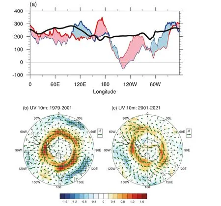
Fig.2.(a) Linear trend of the SLP difference between 40°S and 70°S in 1979–2001 (red; units: pa/10 yr) and 2001–2021 (blue; units: pa/10 yr).The thick lines represent significance at the 90% confidence level.The black line is the SAMI-regressed SLP difference between 40°S and 70°S.Red shading indicates the trend in 1979–2001 is stronger than that in 2001–2021, and vice versa for blue shading.(b, c) Linear trend of the zonal and meridional wind at 10 m (vectors; units:m s- 1 /10 yr) in (b) 1979–2001 and (c) 2001–2021.Shading represents the linear trend of the zonal wind (units: m s- 1 /10 yr).Horizontal and vertical hatching denotes significance at the 90% and 95% confidence level, respectively.
The SAM is closely linked with the Southern Hemisphere extratropical surface climate.The SLP gradient between the middle and high latitudes, measured by the SLP difference between 40°S and 70°S, is directly influenced by the SAM.A positive SAM is related to a stronger SLP gradient, which is true for all longitudes ( Fig.2(a) ).The SLP gradient for all longitudes increases in the ozone depletion era ( Fig.2(a) ).Then, from the beginning of the ozone recovery in 2001, the positive trend in the SLP gradient weakens or slows down at most longitudes( Fig.2(a) ).For example, in 1979–2001, the trend in the SLP gradient at around 60°E is ∼260 Pa/10 yr, while that in 2001–2021 is only∼130 Pa/10 yr.Consistently, the positive trend in midlatitude westerlies is obviously weaker in 2001–2021 ( Fig.2(c) ) than that in 1979–2001( Fig.2(b) ).Fig.2 suggests that the positive trend in the SLP gradient between the middle and high latitudes and the positive trend in the midlatitude westerlies also slows down, but the signs of the trends remain the same and no opposing trends are apparent.
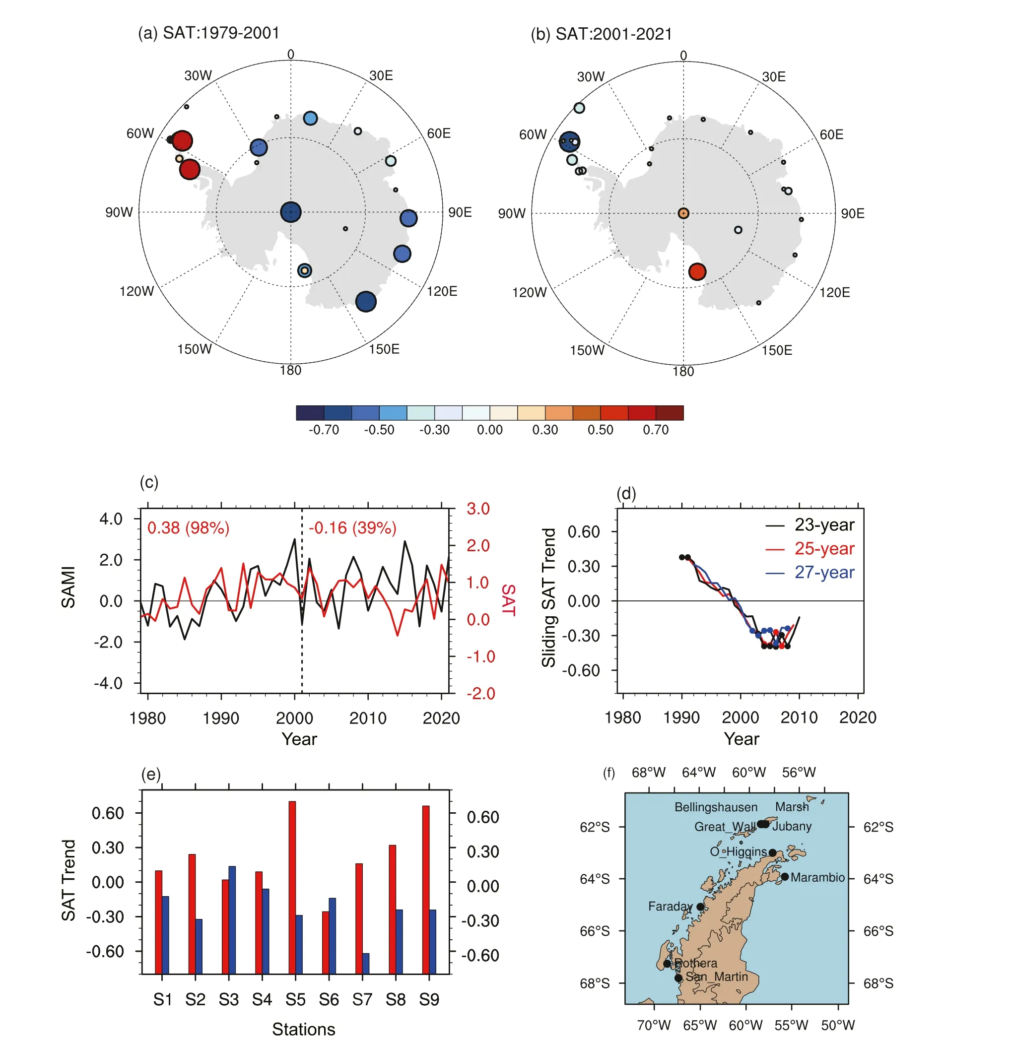
Fig.3.(a, b) Linear trend of the SAT (°C/10 yr) in (a) 1979–2001 and (b) 2001–2021 derived from the least-squares method.Both the color and the circle size are used to represent the strength of the linear trend.(c) Time series of SAMI (black) and the average SAT of nine stations in the Antarctic Peninsula (red; units: °C).The red numbers are the SAT trends in 1979–2001 and 2001–2021, with confidence levels shown in brackets.(d) Sliding trend of the average SAT of nine stations in the Antarctic Peninsula, with sliding windows of 23 (black), 25 (red), and 27 years (blue).Solid circles mean significance at the 95% confidence level.(e) Linear trend of the SAT in 1979–2001 (red) and 2001–2021 (blue) for nine stations in the Antarctic Peninsula derived from the least-squares method.(f) Map of the Antarctic Peninsula showing the locations of the nine stations.
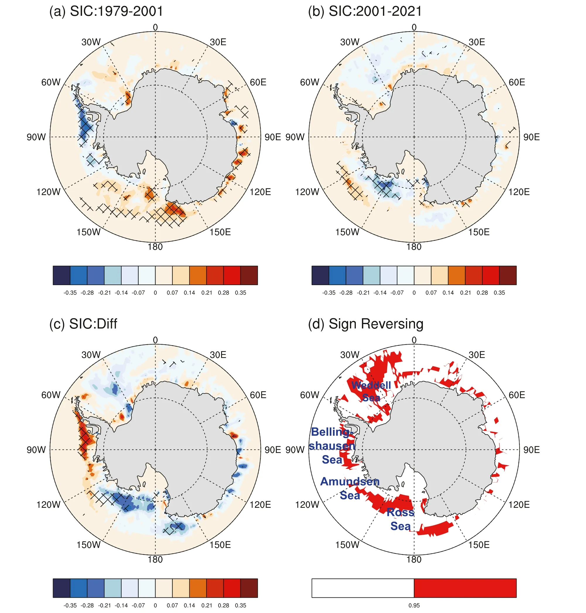
Fig.4.(a, b) Linear trend of the SIC (shading; units: (10 yr)- 1 ) in (a) 1979–2001 and (b) 2001–2021, and (c) the difference between them (shading; units: (10 yr)- 1 ).Hatching indicates significance at the 95% confidence level.(d) The consistency in sign of the linear trends in the two periods.Red shading means the signs of trends in the two periods are opposite.
Fig.3 shows the Antarctic SAT trend.As extensively studied, a positive phase of the SAM warms the Antarctic Peninsula, because stronger summer westerly winds reduce the blocking effect of the Peninsula and cause the formation of a föhn wind ( Marshall et al., 2006 ; Turner et al.,2016 ).The warming in the Antarctic Peninsula from 1979 to 2001 is evident ( Fig.3(a) ).In particular, the warming rates at Marambio station(S5) and San_Martin station (S9) are ∼0.6 °C/10 yr ( Fig.3(e) ).Different from SAMI and the related SLP gradient and westerlies, in which the signs of trends slow down but do not reverse after the ozone recovery,the signs of SAT trends in the Antarctic Peninsula have reversed.There is a cooling trend in the Antarctic Peninsula from 2001 to 2021 ( Fig.3(b) ).The cooling trend at Marambio station (S5) and San_Martin station (S9)is approximately - 0.3 °C/10 yr ( Fig.3(e) ).The time series of the average SAT of the nine stations on the Antarctic Peninsula is shown in Fig.3(c).The trend from 1979 to 2001 is 0.38 °C/10 yr, with the confidence level of 97%, while that from 2001 to 2021 is - 0.16 °C/10 yr.Although the cooling trend in the Antarctic from 2001 to 2021 is not significant, the signs of the SAT trends have reversed from a warming to cooling trend.Similar results were obtained from ERA5 using 2-m air temperature (not shown).The differences in SAT trends between the two periods are significant at the 95% confidence level, via the Chow test illustrated in Section 2.The reversing trend of the Antarctic Peninsula SAT is clear in Fig.3(d) , which shows the sliding trend of SAT using a shorter time length of 23, 25, and 27 years, and the negative SAT trend becomes significant at the 95% confidence level.
Similar analysis is carried out for Antarctic SIC ( Fig.4 ).A positive SAM trend corresponds to a deepening of the Amundsen Low, a climatological low-pressure center located over the Amundsen Sea, leading to warm (cold) air advection to the Bellingshausen Sea (Ross/Amundsen Seas), and thus resulting in melting (increasing) SIC anomalies in the Bellingshausen Sea (Ross/Amundsen Seas) ( Zhang and Li, 2023 ).From 1979 to 2001, during which the SAM shows a strong positive trend,the melting sea ice in the Bellingshausen Sea and increasing sea ice in Ross/Amundsen Seas are evident in Fig.4(a).However, against the background of ozone recovery, the melting of the Bellingshausen Sea disappears and turns into a weak increasing trend, and the increasing sea ice around the Ross/Amundsen Seas changes to a decreasing trend( Fig.4(b) ).The differences in SIC trends between the two periods are shown in Fig.4(c) , and the changes in SIC between 1979 and 2001 and 2001–2021 in the Bellingshausen Sea and Ross/Amundsen Seas are significant at the 95% confidence level via the Chow test.In most regions where sea ice shows a clear response to the SAM, the signs of SIC trends have reversed ( Fig.4(d) ).
3.Summary and discussion
Depletion of Antarctic stratospheric ozone in the Southern Hemisphere during the late 20th century contributed to a strong positive trend in the SAM.However, Antarctic ozone has been recovering since around 2001 thanks to the implementation of the Montreal Protocol.Here, results show that the widely reported austral summer SAM trend flattened around the year 2001, supporting results from previous model simulations that predicted a weakening of the well-documented positive summer SAM trend.Four SAMIs based on different definitions from different datasets show consistency in this slowdown.
Furthermore, considering the strong positive SAM trend in the late 20th century contributed to warming of the Antarctic Peninsula and melting (increasing) sea ice in the Bellingshausen Sea (Ross/Amundsen Seas), changes in Antarctic SAT and SIC against the background of ozone recovery can be detected.Different from SAMI and the related SLP gradient and westerlies, in which the signs of trends slow down but do not change sign after the ozone recovery, the signs of trends in Antarctic SAT and SIC have been reversed.The warming of the Antarctic Peninsula has turned into a cooling trend, and the melting (increasing) of sea ice in the Bellingshausen Sea (Ross/Amundsen Seas) has turned into an increasing (decreasing) trend.The differences in SAT and SIC trends in the Antarctic Peninsula between 1979 and 2001 and 2001–2021 are significant at the 95% confidence level via the Chow test.
The changes in SAT and sea ice against the background of the ozone recovery seem to be stronger than those of the SAM, which may be related to the feedback due to the strong coupling among the atmosphere, ocean and ice, or the synergy with internal variability like the tropical Atlantic SST or tropical Pacific SST ( Li et al., 2014 ).Impacts of the SAM on SAT and SIC take place via regulating surface wind.Local atmosphere–sea-ice–ocean feedbacks may considerably amplify the initial response of SAT and SIC triggered by SAM-related wind forcings ( Li et al., 2023 ).For example, Goosse and Zunz (2014) proposed a positive feedback mechanism that may amplify initial SIC anomalies:when the SIC increases, the mixed-layer depth tends to decrease, and this stronger stratification resulting from the presence of sea ice leads to weakened vertical oceanic heat flux and more heat stored in the ocean,which further contributes to the maintenance of higher SIC anomalies.Besides, SIC anomalies can further amplify SAT anomalies in surrounding regions by triggering atmospheric wind anomalies, especially in austral winter ( Turner et al., 2020 ).Additional diagnostic studies with observational and model data could go a long way towards enhancing our understanding of changes in Southern Hemisphere surface climate against the background of continuous ozone recovery in the future.
Funding
This work was supported by the National Key Research and Development Project [grant number 2020YFA0608902 ] and the Natural Science Foundation of Guangdong Province [grant number 2023A1515010889 ].
杂志排行

Atmospheric and Oceanic Science Letters的其它文章
- Comparison between ozonesonde measurements and satellite retrievals over Beijing, China
- Decadal prediction skill for Eurasian surface air temperature in CMIP6 models
- Ascending phase of solar cycle 25 tilts the current El Niño–Southern oscillation transition
- The Tibetan Plateau bridge: Influence of remote teleconnections from extratropical and tropical forcings on climate anomalies
- Anthropogenic influence on the extreme drought in eastern China in 2022 and its future risk
- Effect of different cold air intensities and their lagged effects on outpatient visits for respiratory illnesses in Handan in different seasons