Comparison between ozonesonde measurements and satellite retrievals over Beijing, China

JinqingZhng , , , Yujin Xun , Jinhun Bin , , , Holgr Vöml , Yunshu Zng , ,Zhixun Bi ,Dn Li ,Hongin Chn

a Key Laboratory of Middle Atmosphere and Global Environment Observation, Institute of Atmospheric Physics, Chinese Academy of Sciences, Beijing, China

b College of Earth and Planetary Sciences, University of Chinese Academy of Sciences, Beijing, China

c College of Atmospheric Sciences, Lanzhou University, Lanzhou, China

d National Center for Atmospheric Research, Boulder, CO, USA

e Electronic Engineering College, Chengdu University of Information Technology, Chengdu, China

Keywords:

ABSTRACT The authors built an electrochemical concentration cell ozonesonde and have been launching it weekly from Beijing on the North China Plain since 2013.This study is the first to use ozonesonde measurements collected over Beijing during 2013–2019 to evaluate vertical ozone profiles derived from the Atmospheric Infrared Sounder(AIRS) onboard the Aqua satellite and Microwave Limb Sounder (MLS) onboard the Aura satellite.The total column ozone calculated from the ozonesonde measurements is also compared with retrievals from AIRS and the Ozone Monitoring Instrument (OMI) onboard the Aura platform.Overall, the ozonesonde measurements and satellite retrievals show similar variability in the ozone profiles (with a relative difference mostly < 10%),albeit with a relatively large discrepancy arising at certain levels.The total column ozone derived from the three instruments shows reasonable agreement and similar annual variation.The annual average total column ozone is 351.8 ± 18.4 DU, 348.8 ± 19.5 DU, and 336.9 ± 14.2 DU for the ozonesonde, AIRS, and OMI, respectively.Further comparative analysis of ozonesonde data collected in the future from multiple sites in China will improve the understanding of their consistency with satellite retrievals over different regions in China.

1.Introduction

Atmospheric ozone has a significant impact on human health, atmospheric chemistry, and climate change ( Lefohn et al., 2018 ).At present,ozone concentrations are primarily observed by a ground-based monitoring network in China (e.g., Li et al., 2021 ), which provides limited insight into the upper-layer ozone variability associated with vertical atmospheric variability.Technologies that detect the vertical ozone distribution, such as electrochemical concentration cell (ECC) ozonesondes ( Komhyr, 1969 ), ground-based ozone lidars ( Xing et al., 2017 ),microwave radiometers ( Sauvageat et al., 2022 ), aircraft ( Ding et al.,2008 ), and satellite platforms ( Aumann et al., 2003 ; Waters et al., 2006 ),play an important role in understanding tropospheric ozone variability and stratospheric ozone depletion.Long time series of vertical ozone profiles extending from the ground to ∼35 km in altitude have been provided by hundreds of ozonesonde stations around the world in operation since 1960.These datasets have been widely used to investigate the trends of variation in ozone and evaluate model simulations and satellite retrievals (e.g., Terao and Logan, 2007 ; Bian et al., 2007 ;Thompson et al., 2011 ).

In China, the Institute of Atmospheric Physics (IAP), Chinese Academy of Sciences, successively developed two types of ozonesondes –namely, the Brewer-Mast type GPSO3 ozonesonde ( Wang et al.,2003 ; Xuan et al., 2004 ) and the subsequent IAP ECC ozonesonde( Zhang et al., 2014 ).They have been used since 2001 to conduct ozonesonde observations once per week in Beijing.By using the singlecell GPSO3 data collected during 2002–2005, Bian et al.(2007) assessed coincident vertical ozone profiles retrieved from the Atmospheric Infrared Sounder (AIRS), version 4, onboard the Aqua satellite, and Microwave Limb Sounder (MLS), version 1.5, onboard the Aura satellite,which indicated that both satellite datasets could reproduce the gradients and variability of ozone in the upper troposphere and lower stratosphere (largely with a difference < 10%).Due to the better detection performance of the ECC ozonesonde, this type of ozonesonde was built by the IAP starting in 2013 ( Zhang et al., 2014 ; Zheng et al., 2018 ) to replace the single-cell ozonesonde.The ECC ozonesonde measurements over Beijing have been widely used to study the vertical ozone distribution and trends of variation in ozone at different time scales and altitudinal levels (e.g., Zhang et al., 2020 , 2021 ; Tang et al., 2021 ; Hong et al.,2022 ; Liao et al., 2023 ; Zeng et al., 2023 ).In November 2021, the China Meteorological Administration employed this ozonesonde for pilot operations at five domestic stations (i.e., Beijing, Chongqing, and Nanjing in Jiangsu Province, Qingyuan in Guangdong Province, and Shaowu in Fujian Province).

To date, Beijing station has provided a unique long-term ozonesonde dataset for mainland China, based on which the vertical distribution and trends of variation in ozone have been widely investigated at different time scales (daily, monthly, seasonal, annual, etc.) (e.g., Zhang et al.,2020 , 2021 ; Tang et al., 2021 ; Liao et al., 2023 ).Moreover, clustering techniques have also been applied to Beijing ozonesonde data to characterize the main characteristics of the variation in ozone profiles and explore the forcing mechanisms of the clustering results, such as meteorological and chemical processes, pollutant transport, and stratospheric intrusion ( Liao et al., 2023 ; Zeng et al., 2023 ).

Given that so many studies as listed above have investigated the temporal variability of ozone by using Beijing ozonesonde data, such similar analysis is beyond the scope of this study.The GPSO3 ozonesonde data have been compared with satellite retrievals ( Bian et al., 2007 ).However, in contrast to the wide use of ECC ozonesonde data to study the temporal variability of ozone mentioned above, a comparison between ECC ozonesonde data and satellite products is still lacking, which is therefore the research objective of the current study.Specifically, this study employs ECC ozonesonde measurements collected from Beijing during 2013–2019 to compare, for the first time, with satellite-retrieved vertical ozone profiles from AIRS and MLS.Moreover, the total column ozone calculated from the ozonesonde measurements is also compared with that retrieved from AIRS and the Ozone Monitoring Instrument(OMI) onboard the Aura platform.

The rest of the paper is organized as follows: the ozonesonde measurement and satellite retrieval datasets are described in Section 2 ; comparisons between the two datasets are presented in Section 3 ; and conclusions are summarized in Section 4.

2.Data and methods

2.1.Ozonesonde measurements

The ECC ozonesonde was routinely launched once a week during 2013–2019 to provide the ozone partial pressure (which is converted to ozone concentration in ppbv in this study) from the ground to a height of∼35 km at the Nanjiao Meteorological Observatory (39.81°N, 116.47°E;31 m in altitude) in Beijing.The release time was ∼1400 CST (China Standard Time, UTC + 8) when the maximum surface ozone concentration and highest mixed layer occurred.The average deviation of the ozone partial pressure originally measured by our ozonesonde and Environmental Science (ENSCI) Corporation produced ENSCI-Z ozonesonde was < 0.3 mPa, and the relative difference in the total column ozone from our ozonesonde and ground-based Brewer spectrophotometer was 6% ( Zhang et al., 2014 ).

The ozonesondes use the 1% full buffered sensing solution type SST1.0 and were prepared following the standard recommendations for ECC ozonesondes.The average background current used in the initial processing was 0.02 ± 0.017μA.The average time to pump 100 ml of air (flowrate time) was 29.6 ± 2.14 s.The average response time measured after the ozone conditioning was 24.7 ± 4.1 s.The ozonesonde data were initially processed using the standard ECC equation (e.g.,Johnson et al., 2002 ).No empirical efficiency correction has been established for the ECC built at IAP.Such empirical efficiency corrections have been well established for the ECC built by Science Pump Corporation (SPC) using the SST1.0 ( Komhyr, 1986 ) and the ECC built by ENSCI using SST0.5 ( Komhyr et al., 1995 ).Instead of determining a new set of empirical efficiency corrections, we reprocessed all profiles using the time response corrections of Vömel et al.(2020).This method attributes the required efficiency corrections at high altitudes and low pressures during a sounding to the time response of the secondary reactions within the ECC.It also considers the time response of the fast primary reactions between potassium iodide and ozone.Laboratory measurements and field data have shown good results replacing the empirical efficiency corrections with the time response correction considering the reaction kinetics within the ECC ( Vömel et al., 2020 ).In the time response correction algorithm, we used a solution efficiency correction factor of 1.08 for the higher buffered SST1.0.The time response constant for the fast KI reaction used the measured response time during the sonde preparation.The time response constant for the slower secondary reactions used a value of 25 min.We used a constant scaling of the cell current of 4% based on the differences between SPC and ENSCI sondes ( Deshler et al., 2017 ).Lastly, we used the measured true pump efficiency corrections of Zheng et al.(2018) , which virtually agree with those of Johnson et al.(2002) and Nakano and Morofuji (2022)( Fig.1 (c)).

The average altitude of the first thermodynamic tropopause above Beijing station is ∼11 km ( Zhang et al., 2021 ), above which the reprocessed ozone concentration is higher than indicated by the original measurements during 2013–2019 for all 307 ozonesonde profiles selected ( Fig.1 (a, b)).Overall, the average difference of all ozone profiles between the original measurements and processed data seem to be distinct between 20 and 35 km ( Fig.1 (d)), which is primarily induced by the pump efficiency corrections ( Fig.1 (c)) in the processed data.

2.2.Satellite retrievals and their collocation with ozonesonde measurements

The vertical ozone profiles derived from the Version 7 Level 3 AIRS and Version 5 Level 3 MLS products are compared with the ozonesonde measurements in this study.To synchronize the vertical resolution of the satellite products, ozonesonde measurements are interpolated onto 20 AIRS pressure levels between 1000 and 5 hPa (i.e., 1000, 925, 850,700, 600, 500, 400, 300, 250, 200, 150, 100, 70, 50, 30, 20, 15, 10,7, and 5 hPa) and 21 MLS pressure levels between 261 and 5.6 hPa(i.e., 261, 215, 178, 147, 121, …, 12, 10, 8.3, 6.8, and 5.6 hPa).The uppermost level of the satellite products is interpolated to the ceiling height of each coincident ozonesonde profile.The local overpass times for AIRS onboard the Aqua satellite are 1330 and 0130 CST, which is 1345 CST for MLS onboard the Aura satellite.The AIRS-based ozone profiles within 1°latitude–longitude around the Beijing site are selected,grouped by day, and averaged for comparison with the ozonesonde profiles collected on corresponding days ( Zhang et al., 2023 ).This spatial collocation criterion is set as 8° for the MLS product given its coarse sampling ( Bian et al., 2007 ).In addition to the vertical ozone profile,this study also compares the total column ozone calculated from the ozonesonde with that retrieved from AIRS and OMI.The ozonesondebased total column ozone is calculated by integrating the ozone up to 10 hPa or balloon burst (whichever comes first) and then using the MLS ozone climatology to estimate the amount of ozone above ( McPeters and Labow, 2012 ; Tarasick et al., 2021 ).

Fig.1.The (a) original measurements from 307 individual ozonesonde profiles collected over Beijing during 2013–2019, and (b) after processing by correction.(c)Pump efficiency corrections from Zheng et al.(2018) applied to the IAP ozonesonde (blue), from Johnson et al.(2002) applied to the SPC-6A (brown) and ENSCI-2Z(yellow) ozonesondes, and from Nakano and Morofuji (2022) applied to Japan Meteorological Agency (JMA) measurements (purple).(d) Comparison of the vertical average ozone of the original measurements (blue) and processed product (red) in Beijing.

3.Comparison between ozonesonde measurements and satellite retrievals

3.1.Vertical ozone profile

Fig.2 compares 285 matched ozone profiles from the ozonesonde and AIRS.The overall pattern of variation in the vertical ozone structure agrees between the two methods ( Fig.2 (a, b).Specifically, the relative difference of each profile ( Fig.2 (c)) indicates that, compared with the ozonesonde, AIRS widely retrieves lower ozone values near the surface, and, upward from 700 hPa, larger values are consistently presented by AIRS in the troposphere below 300 hPa.Additionally, AIRS seems to frequently underestimate the ozone between 300 and 100 hPa;however, at numerous pressure levels above 100 hPa, AIRS tends to detect higher ozone concentrations.In general, the vertical average of all matched profiles is consistent between the two methods ( Fig.2 (d),mostly with a relative difference of < 10%), which is similar to the agreement presented by Fu et al.(2018) who used ozonesonde data from the World Ozone and Ultraviolet Radiation Data Centre collected in 2006.To be more precise, however, the AIRS retrieval is commonly higher than the ozonesonde measurements below 300 hPa.The tropospheric ozone, especially in the boundary layer, is primarily generated by photochemical reactions involving NOxand volatile organic compounds ( Vermeuel et al., 2019 ) and exhibits distinct spatial variability.The ECC ozonesondes used in this study are mostly released at ∼1400 CST from the Beijing site and the spatial coverage of the ozonesonde profile varies due to the balloon’s drift, whereas the satellite products are generally averaged over a wider spatial coverage on the ozonesonde day.A certain spatiotemporal inhomogeneity between the ozonesonde measurements and satellite retrievals may affect their agreement.Although the pump efficiency corrections in Zheng et al.(2018) are applied to the ozonesonde measurements, they still underestimate the ozone concentration above 10 hPa as compared with the AIRS retrieval.Further investigations based on more laboratory tests and field experiments are still needed to acknowledge and solve the deficiency of ozonesonde measurements above 10 hPa.

Fig.3 displays a similar comparison as described above but for the 245 matched ozone profiles from the ozonesonde and MLS.Again, the general pattern of variability identified by the two methods is consistent ( Fig.3 (a, b)).However, a closer look at their relative differences( Fig.3 (c)) reveals that the ozone values from the MLS below 100 hPa appear to alternate between higher and lower values when compared to the ozonesonde.Nevertheless, their agreement improves between 100 hPa and 10 Pa, above which lower ozone is universally measured by the ozonesonde.The average vertical profiles of the ozonesonde and MLS ( Fig.3 (d)) are highly consistent from 215 hPa to 10 hPa (with a relative difference < 10%).In contrast, higher ozone is detected by MLS at its bottom pressure level (261 hPa), and a deficiency is exhibited by ozonesonde measurements above 10 hPa, as mentioned above.In this study, both the ozonesonde instrument and data processing method have been improved when compared to previous studies (e.g.,Bian et al., 2007 ).For the GPSO3 ozonesondes used in Bian et al.(2007) ,the difference was generally within 10% in the upper troposphere and lower stratosphere (from 400 to 70 hPa), and was 20%–30% in the middle troposphere as compared to AIRS, which was 20% in the lower stratosphere and 30% in the upper troposphere as compared to MLS.The updated ECC ozonesonde and data processing method used in this study result in a difference of mostly < 10% relative to the satellite retrievals(both AIRS and MLS) at their product pressure levels.

3.2.Total column ozone

Fig.4 presents the density scatter of the total column ozone derived from the ozonesonde measurements and satellite retrievals.Overall, the results from the ozonesonde and AIRS exhibit reasonable agreement( Fig.4 (a)), as shown by most data points falling along the 1:1 line.The correlation coefficient (R), mean bias error (MBE; sonde minus AIRS),and root-mean-square error (RMSE) between the two datasets are 0.87,3.54 DU, and 21.11 DU, respectively.Similarly, the majority of the data points from the ozonesondes and OMI also fall along or overlap the 1:1 line ( Fig.4 (b)); theirR, MBE, and RMSE are 0.86, 13.67 DU, and 24.51 DU, respectively.

A comparison of the annual variability in total column ozone is shown in Fig.5.Overall, the ozonesonde, AIRS, and OMI data demonstrate similar annual patterns of variability.It should also be noted that the ozonesonde measurements generally agree with the AIRS data,which is higher than the OMI data.The annual average total column ozone is 351.8 ± 18.4 DU, 348.8 ± 19.5 DU, and 336.9 ± 14.2 DU for the ozonesonde, AIRS, and OMI, respectively.

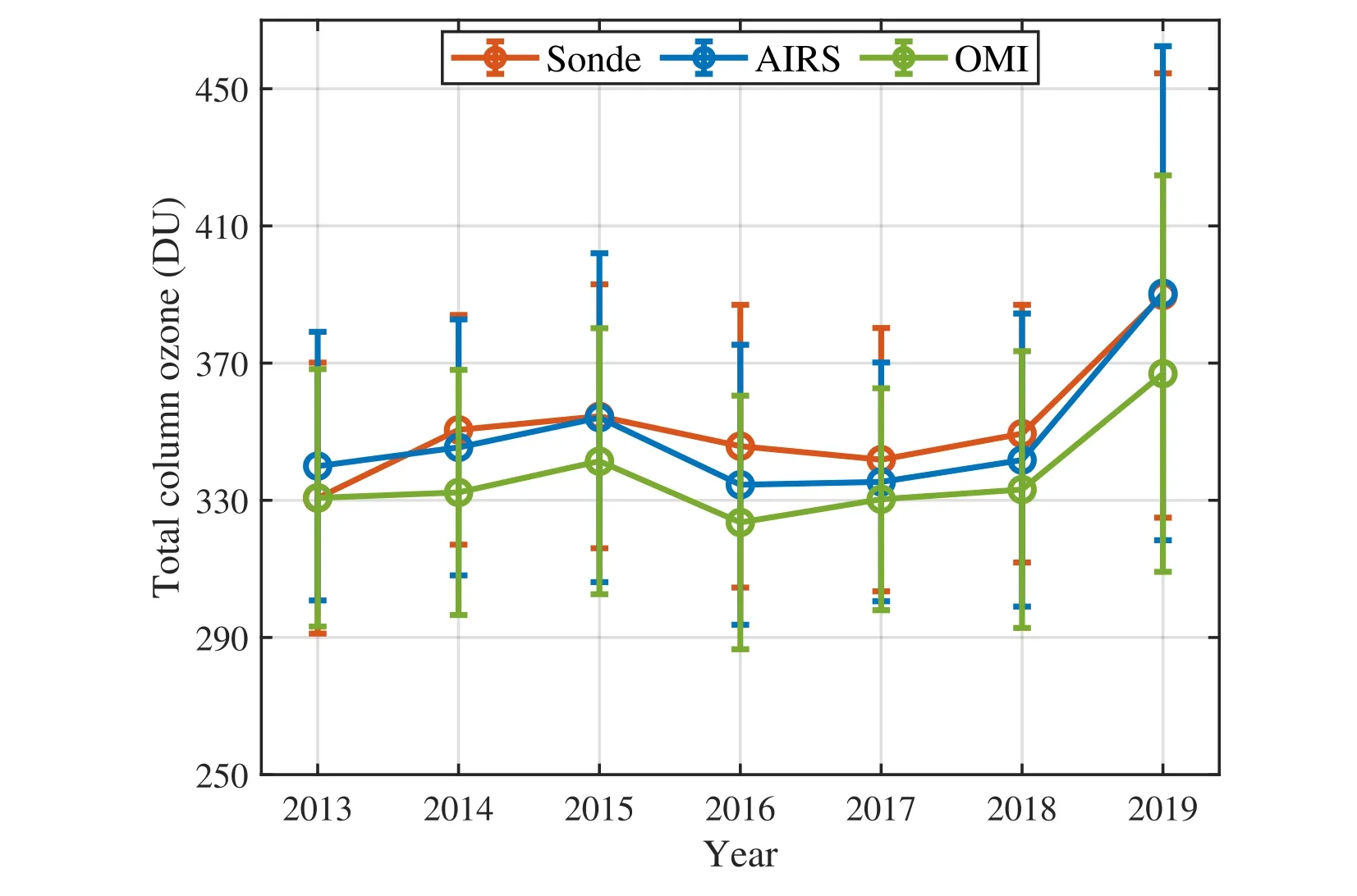
Fig.5.Annual variability in total column ozone and its standard deviation from ozonesonde measurements (brown) and AIRS (blue) and OMI (green) satellite retrievals.

4.Conclusions

The ozonesonde station at Beijing has provided a unique long-term ozonesonde dataset for mainland China.In this study, ozonesonde measurements collected in Beijing during 2013–2019 are used to evaluate space-borne retrievals of vertical ozone profiles from AIRS and MLS and the total column ozone from AIRS and OMI.In general, the vertical ozone profiles between the ozonesonde and space-borne AIRS and MLS agree (mostly with a relative difference of < 10%); however, a relatively larger discrepancy also arises at more detailed levels, such as an overestimation in the AIRS data below 300 hPa, an overestimation in the MLS data at the lowest pressure level (261 hPa), and a deficiency of the ozonesonde measurements above 10 hPa.The total column ozone exhibits reasonable agreement between the ozonesonde measurements and satellite retrievals.TheR, MBE, and RMSE are 0.87, 3.54 DU, and 21.11 DU for between the ozonesonde and AIRS; and 0.86, 13.67 DU,and 24.51 DU for between the ozonesonde and OMI.The annual average total column ozone is 351.8 ± 18.4 DU, 348.8 ± 19.5 DU, and 336.9 ± 14.2 DU for the ozonesonde, AIRS, and OMI, respectively.The ECC ozonesondes used in this study are mostly released at ∼1400 CST from the Beijing site and the spatial coverage of the ozonesonde profile varies due to balloon drift, which will induce a certain spatiotemporal inhomogeneity between the ozonesonde measurements and satellites retrievals and thus may affect their agreement.The ECC ozonesonde measurements from Beijing are compared with satellite retrievals in this study.Future studies based on the data collected by ECC ozonesondes from pilot programs located at multiple sites will help in better understanding their consistency with satellite retrievals over different regions in China.

Funding

This work was supported by the National Natural Science Foundation of China [grant numbers 42293321 and 41875183 ].

Acknowledgments

The authors appreciate the assistance of the Beijing Nanjiao Meteorological Observatory with the ozonesonde launches.We extend thanks to Xiaowei Wan for launching the ozonesonde in Beijing.The AIRS and MLS products are available online from https://disc.gsfc.nasa.gov/.OMI data are available online from https://avdc.gsfc.nasa.gov/pub/data/satellite/Aura/OMI/V03/L2OVP/OMTO3/.