Analysis of pressure response at an observation well against pressure build-up by early stage of CO2 geological storage project

Qing Sun ,Kyuro Sski ,Qinxi Dong ,Zhenni Ye ,Hui Wng ,Hun Sun

a School of Civil Engineering and Architecture,Hainan University,Haikou,570228,China

b Faculty of Engineering,Kyushu University,744 Motooka,Nishi-ku,Fukuoka,819-0385,Japan

c Key Laboratory of Equipment Safety and Intelligent Technology for Guangzhou Rail Transit System,Guangzhou,510430,China

Keywords:CO2 storage Saline aquifer Observation well Pressure response CO2 saturation

ABSTRACT To ensure a safe and stable CO2 storage,pressure responses at an observation well are expected to be an important and useful field monitoring item to estimate the CO2 storage behaviors and the aquifer parameters during and after injecting CO2,because it can detect whether the injected CO2 leaks to the ground surface or the bottom of the sea.In this study,pressure responses were simulated to present design factors such as well location and pressure transmitter of the observation well.Numerical simulations on the pressure response and the time-delay from pressure build-up after CO2 injection were conducted by considering aquifer parameters and distance from the CO2 injection well to an observation well.The measurement resolution of a pressure transmitter installed in the observation well was presented based on numerical simulation results of the pressure response against pressure build-up at the injection well and CO2 plume front propagations.Furthermore,the pressure response at an observation well was estimated by comparing the numerical simulation results with the curve of CO2 saturation and relative permeability.It was also suggested that the analytical solution can be used for the analysis of the pressure response tendency using pressure build-up and dimensionless parameters of hydraulic diffusivity.Thus,a criterion was established for selecting a pressure transducer installed at an observation well to monitor the pressure responses with sufficient accuracy and resolution,considering the distance from the injection well and the pressure build-up at the injection well,for future carbon capture and storage (CCS) projects.

1.Introduction

The average atmospheric CO2concentration had increased from 280 ppm in industrial era to 411 ppm in May 2019(Lake and Lomax,2019).The average CO2concentration is increasing continuously by more than 2 ppm/year(Metz et al.,2005).With this growth rate,it will exceed 450 ppm within the next 20 years (Li et al.,2019),and the mean global temperature will increase by over 2°C.To mitigate the increasing rate,many intergovernmental organizations have assessed climate change and exchange technology for reducing the anthropogenic CO2emissions (Metz et al.,2005;Shackley et al.,2005;IEAGHG,2010).In 2017,a possible framework to reduce CO2emissions into the atmosphere had been agreed upon countries that joined COP23 (Obergassel et al.,2018).

CO2capture and geological storage is a promising way to mitigate CO2emissions into the atmosphere by capturing CO2gases from relatively large industrial sources,such as power plants,and then transporting and injecting them into porous and permeable storage reservoirs.A suitable reservoir should be covered by sealing layers with very low permeability to prevent CO2leakage from storage reservoirs to the ground surface or sea bottom.Three main underground storage reservoirs have been identified: saline aquifers,depleted oil and gas reservoirs,and unminable coal seams(Yang et al.,2010).Deep saline aquifers at depths over-800 m have been considered ideal because of their large storage capacity and broad distribution worldwide.The saline aquifers are permeable geologic layers located 1000-3000 m deep and can store injected CO2in a supercritical state under reservoir conditions.

The International Energy Agency (IEA) has estimated the potential contribution of carbon capture and storage (CCS) in mitigating global CO2emission to be as high as 20% of the global emissions in 2050,which follows the most important contribution by improvement in energy efficiency (Lipponen et al.,2011).The Blue Map reduction plan has been considered necessary to continue annual geological storage of 9.5 Gt-CO2by CCS for 45 years.Several ongoing pilots and commercial CCS projects have suggested that CO2geological storage in deep sedimentary formations is technologically feasible(Eiken et al.,2011;Hansen et al.,2013;Tanaka et al.,2014).To make a significant contribution to the mitigations of climate change,many CCS projects with larger CO2injection rates from an injection well need to be planned and implemented.However,the CO2reduction rate by CCS projects is currently limited because sufficient CCS projects have not been implemented owing to economic issues as well as social acceptance issues related to storage safety and stability.

CO2injections induce a pressure increase in the reservoir from its original geomechanical pressure.A large CO2injection rate can easily cause considerable pressure build-up in the bottom hole and its surrounding region in the reservoir,where activated faults through the upper sealing layers may lead to CO2leakage(Rutqvist,2012;Mathias et al.,2014;Harp et al.,2017;González-Nicolás et al.,2019).Therefore,the management of the bottom hole pressure(BHP)as an induced pressure build-up will be a critical factor in the safe operation of CO2storage (Buscheck et al.,2012;Yang et al.,2018;Zheng et al.,2022).For instance,the In Salah CCS project in Algeria has shown significant geomechanical changes because of the injection pressure and site-specific geomechanical conditions.Although the injection rate of the In Salah CCS project was 1 Mt/year,the project was still shut down because of concerns about the integrity of the seal layers(Eiken et al.,2011;Goertz-Allmann et al.,2014).In the Tubåen Formation in the Snøhvit field (offshore Norway),Statoil successfully injected 1.6 Mt of CO2from April 2008 to April 2011.However,the CO2injection had to be stopped owing to an increase in pore pressure before reaching the full storage capacity of the Tubåen Formation (Hansen et al.,2013).It is easy to induce tremendous pressure build-up in the reservoir at a large injection rate.All the site CCS programs teach us that formation pressure monitoring and management is a key point to limit the implementation of CCS program on a commercial scale.

Generally,to confirm that the injected and stored CO2is in a safe and stable condition,it is necessary to grasp the behavior of CO2in the reservoir and to detect whether there is leakage of CO2out of the reservoirs or not.For example,in the Tomakomai CCS demonstration project(hereinafter Tomakomai CCS project)(Tanaka et al.,2014),five continuous monitoring items and three periodic monitoring items were operated for two aquifers at different average depths of 1150 m and 2700 m.The continuous monitoring items are temperature and pressure in two injection wells,temperature and pressure in two remote observation wells,and seismic monitoring at the ocean bottom and onshore.In contrast,the periodic monitoring items are marine environmental observations (sea water,bottom mud,and sea lives) and two-dimensional and threedimensional seismic surveys.Specifically,two observation wells were drilled from onshore to the Moebetsu Formation (1100-1200 m in deep) and the Takinoue Formation (2400-3000 m in deep)to record continuous passive changes in aquifer pressure and temperature as well as CO2saturation in each formation water.The monitoring data recorded in the observation wells can be used to detect the movement of the CO2plume and judge the stability of stored CO2based on comparisons with the numerical simulation results using aquifer models.The original pressure of the Moebetsu Formation at the injection well was 9.3 MPa and the maximum BHP in the injection well that was recorded during the test injection was 10 MPa (Tanaka et al.,2014;Sato and Horne,2018;Sawada et al.,2018).However,there is no pressure response recorded in the observation well OB-2(Tanaka et al.,2014)which was drilled about 3000 m from the injection well in the Moebetsu Formation with installing pressure and temperature sensors.The reason for the lack of pressure response at the observation well was explained as the sensitivity of the pressure transducer is not sufficient to detect the pressure propagation from the injection well to the observation well.

Generally,observation wells are drilled to observe the aquifer with CO2storage.It is assumed that temperature and pressure gauges are installed in the bottom hole for continuous monitoring of the aquifer.They are used to detect the CO2plume front development and verify that the injected CO2had not leaked into shallower strata (Metz et al.,2005).Most of the observation wells are used to monitor the CO2plume front position (Mathieson et al.,2011;Hu et al.,2015).The In Salah CCS program used an observation well KB-5(Durucan et al.,2011)with a distance of 1.3 km from the injection well KB-502 and analyzed the gas tracer injected together with CO2to examine the CO2plume development.The observation well KB-5 was used for detecting the CO2plume position,not for the pressure analysis,and it was an abandoned gas production well drilled in 1980,which was not well designed for the CCS program.In Germany,a Ketzin pilot CCS program used two observation wells(Ktzi 200 and Ktzi 202)to determine the pressure evolution during injection operation with a distance of 50 m and 112 m from the injection well Ktzi 201 (maximum injection rate 78 t-CO2/d),respectively (Liebscher et al.,2013).If the distance between the observation wells and the injection well is extremely small,it can detect the CO2plume front development.However,according to some in situ experience,the greatest risk of CO2leakage for any geological storage project is associated with old wells and observation wells.Thus,an observation well located at a small distance from the injection well also creates a new potential pathway for CO2leakage to the sublayers.

Drilling a new observation well requires an additional budget and may create a new potential pathway for CO2leakage to the surface.Therefore,the observation well and installed sensors for measuring parameters,such as distance from the CO2injection well and the sensor sensitivity,should be suitably designed before drilling an observation well.In this study,we numerically investigated the pressure response at an observation well,induced by CO2injection at the early stage of CO2geological storage in a deep saline aquifer.The results can be used as reference data for designing an observation well and determining the location for installing sensors(or transmitters).

2.Aquifer model for CO2 injection and storage

As shown in Fig.1,a cylindrical grid system with (r,φ,z) coordinates was used to construct the reservoir model.The pressure and CO2saturation distributions were simulated by injecting CO2from an injection well located atr=0 m into an aquifer with radiusrw.It was assumed that the aquifer had uniform porosity and permeability in horizontal and vertical directions.Its outer boundary atr=reis defined as an open boundary that the pressure is equal to the initial pressure.There is no-flow across the top and bottom boundaries.A typical aquifer model was simulated by settingrw=0.1 m andre=10 km.

The meshing of the aquifer in therandzdirections is shown in Fig.2.The grid blocks consist of 1000×1×10 grid cells in the(r,φ,z) directions,of which 200 grid-cells were set betweenr=0.1-400 m,and 800 grid-cells betweenr=400-10,000 m.The reservoir consists of 10 layers with a constant spacing of 10 m in the vertical direction.CO2was injected from the injector into horizontal layers connecting to the aquifer by three types of perforations.The radial distance from the observation well to the injection well,rm,was assumed to be in the range of 1000-5000 m.The pressure changes in the aquifer blocks connected to the aquifer atr=rmwere considered as the pressure responses at the bottom of the observation well connected to the aquifer.Numerical simulations were conducted using the compositional reservoir simulator CMG-STARS™.

Fig.2.Schematic diagram of meshing in the cross-section.

The simulation parameters for the base model are listed in Table 1.In the case of the Moebetsu Formation in the Tomakomai CCS project,the range of horizontal permeability was estimated ask=0.98 × 10-15-980 × 10-15m2(=1-1000 mD) from the geophysical measurements,andk=363 × 10-15m2(=370 mD)based on the fall-off test using the injection well after drilling.In addition,the porosity was measured as φ=0.2-0.4 by a laboratory core test and the excavation result was φ=0.12-0.42(Tanaka et al.,2014).In this simulation,the uniform permeability in the horizontal direction was also set ask=363×10-15m2,and the ratio of vertical permeability (ky) to horizontal permeability (k) wasky/k=0.1.The porosity φ=0.3 was used for the base simulations.In the present simulations,assuming that the ground surface temperature was 15°C and geothermal gradient as 2.5-2.75°C/100 m,the targeted aquifer temperature was 40°C-42.5°C,and the CO2injection temperature was specified as 40°C.Therefore,the injected CO2was similar to the isothermal process.No geochemical reactions or mineralization were considered because a short period of fewer than 200 d was considered for simulation.In the CMGSTARS™compositional models,the phase equilibrium is specified via phase equilibrium ratios,K-value,which is a function of gas phase pressure and temperature.

Table 1Aquifer parameters and CO2 injection well set in the base model(Tanaka et al.,2017;Sawada et al.,2018;Garimella et al.,2019).

Relative permeability was modeled based on the Brooks-Corey-Burdine model (Garimella et al.,2019) and is expressed by

whereSeis the effective saturation;krwandkrgare the aqueous and gas phase relative permeabilities,respectively;Swis the aqueous phase saturation;SwrandSgrare the aqueous and gas phase residual saturations,respectively;and λ is the pore size distribution index.In the present simulations,Swr=20%,Sgr=5%,and λ=0.5.The relative permeability curves are shown in Fig.3.Based on the curves,the remaining water saturation after displacement of CO2gas is almostSw≈65%,which means that the CO2gas saturation becomesSg≈35%in an aquifer except near the well.

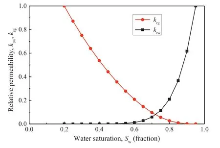
Fig.3.Relative permeability curves used in present simulations (Brooks-Corey-Burdine model) (Garimella et al.,2019).

3.Theoretical analysis

3.1.Linearized radial flow equation and estimation solution

Assuming that porous media are viscous-dominated and there is no turbulent flow,the flow in porous media can be described by Darcy’s law for a single incompressible fluid phase(Hubbert,1953):

where q is the vector of the volumetric flow rate (m3/s);k(m2) is the permeability;μ (Pa s) and ρ (kg/m3) are the viscosity and density of the reservoir fluid,respectively;g is the gravitational acceleration vector directed downwards;and ∇pis the hydraulic gradient.

Without considering gravity in the vicinity of an injection well,the governing equation on pressurep(Pa) for one-dimensional radial linearized flow,assuming a constant compressibility in the aquifer,is given as (Wu and Pan,2005):

whereCt=Cr+Cf(Pa-1) is the total value of rock compressibility(Cr)and reservoir fluid compressibility(Cf),andt(s)is the elapsed time from the start of CO2injection.The hydraulic diffusivity,η,is a hydraulic parameter that controls the unsteady pressure transient.

The pressure build-up in an injection well,defined aspi,under the general steady-state radial flow is proportional to the fluid injection rateq(m3/s),while it is inversely proportional to the transmissivity (or permeability-thickness product)K=kH(m3),which is product of the horizontal permeabilitykand the reservoir thicknessH(m) (Dietz,1965).The transmissivityKexpresses the flow capacity and ability in aquifers and reservoirs.The radial flow solution for the steady-state (∂p/∂t=0) in Eq.(6) is given by the following equation (Van Everdingen and Hurst,1949;IEAGHG,2010):

wherere(m) is the effective reservoir radius,which is the extent from the injection well to the reservoir boundary where the pressure is equal to the initial hydrostatic pressure;andrw(m) is the injection well radius.

Assuming that the reservoir fluid is uniform and uncompressible (Cf=0 and ρ=const.),a typical solution of radial transient flow can be expressed as (Goode and Thambynayagam,1987):

wherep0is the initial or outer boundary pressure of the aquifer,and μq/(4πkH)is a constant for a constant if the injection rateqis set as a constant without considering skin factors.This solution shows the reservoir pressure build-up at different injection periods and different radial distances from the injection well.The transient pressure changes in the aquifer at the elapsed time from the start of injection are expressed by the transient flow equation and are shown in Fig.4.

Fig.4.Schematic solution showing transient pressure for pressure build-up at an injection well.

The pressure response at the observation well atr=rm,Δp(Pa),can be estimated by

The pressure calculated by Eq.(8) is roughly equal to the pressure changes between build-up and fall-off atr=rm.The transient condition is applicable only if the pressure response in the aquifer is assumed to be not affected by the presence of the outer boundary;thus,the reservoir appears infinite in extent.In this study,a constant pressure boundary was assumed to be close to an aquifer with enough radius.Therefore,it is possible to use this equation to estimate the rough pressure response at the observation well.

The distance from the CO2injection well to the observation well(r=rm)is the critical parameter that controls the magnitude of the pressure response at the observation well,which is affected by the CO2injection rate and amount from the injection well and the aquifer parameters.According to Eq.(7),the magnitude of the response pressure is directly proportional to the injection rate,q,and injection period,while the transmission delay time is inversely proportional to the hydraulic diffusivity of the aquifer.The pressure response is almost inversely proportional to distancerm.

3.2.Analysis method

The initial pressure of the aquifer was set asp0=10 MPa in the present simulations.The BHP in the injection well is equal top0+pi.The pressure response and distribution of CO2saturation in the aquifer were simulated for a constant CO2mass injection rateqm(t-CO2/d) as shown in Fig.5.

Fig.5.Schematic diagram of defined variables.

When the injection well is shut-in after the CO2injection for a period,ti,the pressure response of the observation well changes and has a peak value Δpmax,which is recorded after the delay time,Δtmaxfrom the shut-in of the injection well.A pressure response Δpmaxis sensitive to the magnitude of pressure build-uppi.Therefore,it is expected that the ratio of both pressures defined as

is not sensitive to injection rateq.Simulations were carried out to investigate the pressure response and the delay time of the peak pressure in the observation well by comparing the CO2plume front position extending outward.In the present simulations,the CO2injection rateqwas controlled according to the BHP,which must be less than the threshold capillary pressure and sufficiently less than the fracture pressure of the caprock or upper sealing layer.The maximum BHP has been set as 90% of the threshold capillary pressure (12.6 MPa=14 MPa × 0.9) measured for the Moebetsu Formation (Osiptsov,2017).In the base model,the CO2mass injection rate was set asqm=600 t-CO2/d (q=3.744 m3-std/s,ρCO2=1.855 kg/m3at the surface condition).The injection period in the base model was assumed to beti=100 d,and the distributions of the pressure response and CO2saturation were simulated untilt=1000 d from the start of CO2injection.

4.Pressure build-up at the injection well and pressure response at the observation well

4.1.Effect of perforation scheme for injecting CO2

The CO2injection well was assumed to be a vertical well.As different perforation schemes will lead to a difference in pressure build-up at the well,the effects of the perforation scheme on the CO2injectivity were discussed.As shown in Fig.6,some previous studies used different simulation models with several perforation points and locations for CO2injection(Cinar et al.,2008;Chadwick et al.,2009).In this study,the multiple perforation scheme using 10 holes perforated in the center of each layer (Fig.6a) was used.Chadwick et al.(2009) used the scheme with an injection point located 10 m below the aquifer ceiling (Fig.6b) to study the pressure build-up at the injection well and pressure distribution in the aquifer.Cinar et al.(2008)used the scheme with the injection point located in the middle of the reservoir (Fig.6c).

Fig.6.Injection well perforation schemes used in previous studies: (a) Multiple perforations,(b)Single perforation hole at the top used by Chadwick et al.(2009),and(c)Single perforation hole at a position used by Cinar et al.(2008).

Fig.7 shows the pressure build-up at the injection well with different perforation schemes for CO2injection using the same injection rate.It can be seen that the injection with one perforation point will lead to a significant pressure build-up in the first hour of injection,which is more than twice that of all the perforations(Fig.6a).In the multiple perforation scheme,a larger contact area with the reservoir results in a smaller pressure build-up and less stress on the sealing layer for the same injection rate.Furthermore,only one block in the vertical direction may not be rigorous to study the pressure build-up.If the pressure gradient of the reservoir is not considered,the calculated BHP may be overestimated.Therefore,in this study,a multiple perforation scheme was used in the simulations to ensure a safe injection with a smaller pressure build-up at the well.

Fig.7.Numerical simulation results on pressure build-up of the injection well obtained with different perforation methods of the CO2 injection well using CMGSTARS™.

4.2.Pressure build-up and bottom-hole pressure

To study the pressure build-up at the CO2injection well,an injection scheme based on the base model for injection rateqm=600 t-CO2/d and continuous injection for 100 d (ti=100 d)was simulated compared with the case of injecting saline water that is the same with the reservoir fluid.Injecting CO2and saline water will show the same volume flow rates in the reservoir condition.

After the start of injecting CO2into the aquifer,CO2saturation around the injection well increased with replacing saline water.Therefore,with increasing CO2saturation,the viscosity μ of the aquifer fluid,especially around the injection well,gradually changed from the viscosity of saline-water(μbrine≈6×10-10Pa s)to that of supercritical-CO2viscosity(μCO2≈0.429×10-10Pa s).As shown in Fig.8,a decrease in the transient pressure after a pressure build-up of 350 kPa was observed during CO2injection at a constant injection rate,while the pressure build-up during saline water injection gradually increased.However,at the early stage of CO2geological storage,the magnitude of pressure build-up(≈350 kPa)is similar even if different fluids are injected,because the CO2storage area is limited around the well.Moreover,CO2saturation is also limited to less than 35%,based on the relative permeability curves shown in Fig.3,when CO2dissolution into saline water is neglected.Therefore,the pressure change (≈50 kPa) during the CO2injection period (100 d) is not proportional to the fluid viscosity,even if the viscosity of CO2is less than 10%of the viscosity of saline water.Thus,using the viscosity of saline water in Eq.(6)instead of that of CO2shows a more realistic estimation of the pressure build-up in the aquifer at the initial injection stage.However,the pressure build-up estimated by Eq.(6) using the viscosity of saline water is slightly overestimated than that of CO2.This difference can also be explained by the equation presented by Cinar et al.(2008) and IEAGHG (2010).They modified Eq.(6) by introducing the relative permeability of CO2.However,introducing CO2relative permeability is another complicated question as CO2relative permeability changes with continuous injection,adding more uncertain variables.In this study,the viscosity of saline water is used to estimate the rough pressure build-up using Eq.(6).

Fig.8.Pressure build-up by injecting CO2 and saline water vs.elapsed time for the base model.

In the present simulations,the radial flow consisting of saline water and CO2was calculated considering the relative permeability curves for each fraction.Therefore,physical property changes in the blocks including multi-phase flow were simulated automatically in the present simulations using CMG-STARS™.

Fig.9 shows the cross-sectional simulation results for therandzaxes of CO2saturation and CO2plume flux vectors att=10,50,100 and 200 d after the start of CO2injection.The CO2plume expands mainly as a radial flow,because the horizontal permeability,k,or hydraulic diffusivity,η,is 10 times larger than that of the vertical value.The buoyancy force on unit CO2volume (roughly 4000 kN/m3) induces vertical CO2convection flow,because of the density difference between injected supercritical CO2(≈600 kg/m3) and saline water(=1030 kg/m3)in the aquifer.Therefore,the top layer of the aquifer shows the largest expanding CO2seepage flow velocity with the farthest CO2plume front.Most CO2fluids accumulate and trap between caprocks and reservoirs which is widely recognized as structure trapping.This phenomenon makes it easy to build up extremely pressure which will threaten the safety of caprock.The red arrows in Fig.9 show the flow velocity vectors.It is clear that the CO2plume diffuses mainly in the radial direction during the CO2injection period,while the convection in the vertical direction is much slower.After the injection well was shut-in,the driving pressure in the horizontal direction gradually vanished with fall-off pressure,and the vertical buoyancy flow becomes prominent.

Fig.9.Cross-sectional on r and z axes of CO2 saturation and CO2 plume flux vectors at t=10,50,100 and 200 d for the base model.

We defined the CO2plume front position at the top layer,rp,where the CO2saturation isSc=10%.As shown in Fig.10,the plume front is observed atrp=84 m on the 100th day.Fig.10 shows the CO2plume front position,rp,before and after stopping CO2injection att=100 d (=ti).The CO2plume front position,rp,expands almost proportionally tot0.5for 0100 d,the CO2front slowly expands proportionally to 0.1tby buoyancy force on the CO2plume.

Fig.10.CO2 saturation front distribution over time.

The numerical simulation results of the base model for the distributions of the reservoir pressure change from the initial aquifer pressure (p(r)-p0) and CO2saturation (Sc(r)) att=50 and 100 d are shown in Fig.11.

Fig.11.Numerical simulation results of pressure response vs.CO2 saturation at different distances from the injection well.

It can be seen that pressure changes and CO2saturation distributions are correlated in the region of CO2saturationSc>35%,while only a pressure change is observed in the region(r>100 m)with a CO2saturationSc≈0.Assuming the position of the CO2plume front defined bySc=10%,the pressure transmitting speed is two orders of magnitude higher than that of the CO2plume front,because the pressure change is observed without CO2saturation change.

4.3.Effect of CO2 injection rate and aquifer transmissivity on pressure build-up

Fig.12 shows the simulation results of pressure build-up,piat the CO2injection well for injection rate,qm,compared with the estimated line calculated using Eq.(6)by assuming the viscosity of saline water,as discussed in the previous section.The pressure build-up does not show a significant linear relationship with injection rate.As discussed previously,this can be explained by the changing CO2saturation around the injection well,since the relative permeability changes with CO2saturation.The simulation results show that the linearity betweenpiandqmis better and closer to the values estimated by Eq.(6) with a low injection rateqm<600 t-CO2/d than that with a large injection rateqm>1500 t-CO2/d.This is because the higher injection rate results in a faster change in CO2saturation around the injection well.

Fig.12.Numerical simulation results of pressure build-up pi vs.CO2 mass injection rate qm.

We confirmed that the pressure build-up can be correctly estimated using saline water viscosity to be 65% because the CO2saturation around the injection well is close to 35%.This setting will be used to calculate the pressure change in the reservoir below.

CO2injection into the Moebetsu Formation was conducted and the maximum pressure build-up of the injection well (IW-2) was recorded aroundpi=450 MPa at the injection rateqm=600 t-CO2/d and injection timeti=50 d.The thickness of the Moebetsu Formation is approximately 100-200 m which is uncertain and different from the base model set.Simulations were run,and the pressure build-up against different transmissivities of the aquifer was studied.According to the simulation results shown in Fig.11,the transmissivity of the Moebetsu Formation is approximatelyK=2.7 ×10-11m3,and the permeability of the Moebetsu Formation was calculated as 135 × 10-15-270 × 10-15m2,which is different from our base model settingk=363 × 10-15m2that is overestimated according to a comparison between the field pressure data and simulation results.Owing to the short injection period,the fluid flow around the injection well is in an unsteady state.In Fig.13,the pressure build-up at the injection well aftert=1 and 50 d,with respect to aquifer transmissivityK,were compared with those in the steady-state flow (Eq.(6)).As at the early stage of injection,there is a transient effect of pressure buildup at the injection well,and the pressure build-up of the injection well on the 50th d is closer to the steady-state flow than with that on the 1st d.A higher transmissivity aquifer is becoming closer to the calculated pressure build-up,piof steady-state flow.

Fig.13.Pressure build-up, pi (kPa) vs.aquifer transmissivity, kH (m3).

4.4.Pressure fall-off at the CO2 injection well

Opening or shutting off a well causes pressure changes in the CO2injection well.The CCS projects including fall-off data after shut-in can be used to study the aquifer state (Escobar and Montealegre,2008).When the BHP vs.time plots are measured with sufficient precision after the well shut-in,the aquifer in situ permeability and well skin factor can be estimated by analyzing the data.This is similar to the well-testing method widely used in petroleum reservoir engineering.Without considering the skin factor,the pressure fall-off function in the injection well is expressed by the radial transient flow equation(Eq.(7)).The pressurep0should be modified to the instantaneous BHP when the injection well is shut in.Becauseqμ/(4πkH) can be treated as a constant if the injection rateqis constant,the hydraulic diffusivity η can be considered the main parameter controlling the fall-off curve.

In contrast to the conventional method of analyzing pressure fall-off lines,the pressure fall-off time is defined in this study to analyze reservoir conditions and pressure transients.As shown in Fig.14,t0.75andt0.25are defined as the elapsed times to reach 75%and 25% pressure reductions from the build-up pressure after the well shut-in.The pressure fall-off time is defined as (t0.75-t0.25),which shows the period the pressure falls off 50% of the built-up pressure.

Fig.14.Definition of pressure fall-off time after pressure build-up.

In the case of CO2injection in the Moebetsu Formation,Tomakomai CCS project,some pressure fall-off data were recorded after shutting the well,and the fall-off time(t0.75-t0.25)was analyzed at about 5 d based on the BHP data.The numerical simulation results for the fall-off time (t0.75-t0.25) vs.hydraulic diffusivity η for the base model are shown in Fig.15,which includes the results of different porosities (0.1,0.2 and 0.3) and permeabilitiesk(=98×10-15-1960×10-15m2).As the fall-off time for the Moebetsu Formation(dotted line in Fig.15) was 5 d,the hydraulic diffusivity range of the Moebetsu Formation can be estimated as η=2-4 m2/s from the simulation results of(t0.75-t0.25)and hydraulic diffusivity.As the transmissivity of the Moebetsu Formation was matched asK=2.7×10-11m3in the last section,and the thickness is betweenH=100-200 m,porosity φ=0.2-0.4.Therefore,the matrix rock compressibility of the Moebetsu Formation is estimated asCr=0.14 × 10-9-1.11 × 10-9Pa-1.This means that the rock compressibility set asCr=0.9×10-9Pa-1is within the reasonable range compared with the Moebetsu Formation.

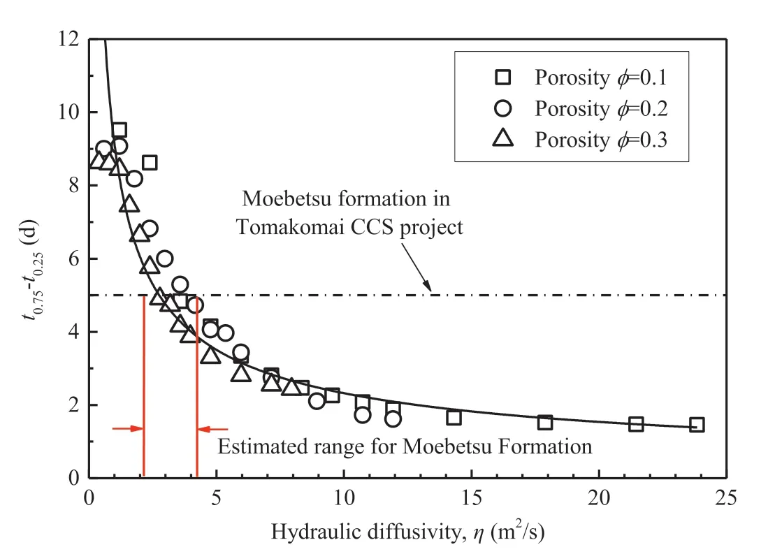
Fig.15.Numerical simulation results of fall-off time (t0.75-t0.25) vs.hydraulic diffusivity η compared with the fall-off time of the Moebetsu Formation (5 d).

4.5.Pressure response at observation wells

In this section,the pressure responses at a hypothetical observation well located at a range of radial distancerm=1000-5000 m from the injection well are discussed based on the simulation results by comparing the values estimated using Eq.(8).The maximum value of pressure response is defined as Δpmax,which is recorded at the observation well (r=rm) after continuous CO2injection forti=100 d in each injection scheme.Fig.16 shows the numerical simulation results of the pressure response at the observation well located atrm=1000,3000 and 5000 m against the CO2injectionqm=600 t-CO2/d forti=100 d (base model).The pressure of the observation well increases gradually during the injection period,which is different from the pressure build-up of the injection well.This is because the pressure build-up in the vicinity of the injection well (less thanr=100 m) is influenced by both CO2and saline water flows,while the pressure disturbance around the observation well far from the injection well is not influenced by the difference in viscosities of CO2and saline water.After the injection well is shut-in (t>ti),the observation well pressure draws a curve similar to the pressure fall-off of the injection well.It can also be seen that there is a time delay between the injection well shut-in to the peak pressure response of the observation well,and this delay time becomes larger as the distance from the injection well increases.The peak value of the pressure response,Δpmaxbecomes smaller and broader,and the peak time recorded at the observation well,Δtmax,increases with increasing distance from the injection well,rm.For example,Δpmax=57 kPa atrm=1000 m becomes more than twice(Δpmax=25 kPa)atrm=3000 m.

Fig.16.Typical simulation results of the pressure response at the observation wells located at rm=1000,3000 and 5000 m.

As shown in Fig.17,the simulation results of Δpmaxhave a linear relationship with the CO2mass injection rateqmand are consistent with the numerical simulation results for injecting saline water.The analytical equation assuming a transient radial flow is expressed as

Fig.17.Numerical simulation results of the pressure response at the observation wells vs.CO2 mass injection rate qm.

The analytical solution obtained with Eq.(10) is less than the simulation results.The difference between the results increases as the radial distance between the injection well and observation wells increases,because the value estimated by Eq.(10)can only be applied for a rough estimation.In this simulation study,the injection period was assumed to beti=100 d,and the peak pressure response at the observation well can be detected after dozens of days.

5.Pressure ratio of injection well and observation well

5.1.Single CO2 injection with pressure build-up and fall-off

To avoid the error in the absolute magnitude of the pressure response at the observation well,we introduced the parameterR,which is the ratio of the pressure build-uppiand the maximum value of pressure response Δpmax.Both the pressure build-up at the injection well and the pressure response at the observation wells have almost linear relationships with the injection rate,qm<600 t-CO2/d.This ratio can be used for determining the pressure response at the observation wells based on the pressure build-up,because the ratioR=Δpmax/piis not sensitive to the mass injection rate,qm.In addition,the termqμw/(4πkH) in Eq.(7) can be treated as a constant if the mass injection rateqmis a constant.Therefore,the value ofRis proportional to the injection period and hydraulic diffusivity but inversely proportional to the square of the radial distance from the well,while it is not as sensitive to the CO2mass injection rateqm.The rough value ofRcan be estimated by the following equation where hydraulic diffusivity,η,is defined by Eq.(5).

whereCtis equal to rock compressibility because fluid is assumed to be incompressible (Cf=0),re=10,000 m is the effective reservoir radius,andrw=0.1 m is the radius of the injection well.Eq.(11)shows thatRconsists of a logarithmic function of timet,aquifer area up to the inner area of the observation well radiusand hydraulic diffusivity,η.Assuming that the observation well response to the peak pressure value occurs at the moment the injection well is shut-in,the timetin Eq.(11) is replaced withti.

The numerical simulations ofRusing CMG-STARS™were performed for the base model with the horizontal permeability range fromk=196 × 10-15-784 × 10-15m2(=200-800 mD),the observation well locationrm=1000-5000 m,and different injection periodsti=50-300 d;the porosity and compressibility of the porous media were considered constant (φ=0.3 andCt=1.4×10-9Pa-1).A sensitive study of hydraulic diffusivity η was also carried out by setting the constant injection rateqm=600 t-CO2/d.The simulation results ofRcompared with values calculated by Eq.(11)are shown in Fig.18.It can be seen that the pressure ratioRshows an almost logarithmic function of ηt/.However,there is a slight difference between the values ofRfor different permeabilities,especially when ηt/>10.Because there is a time delay between the injection well shut-in and the observation well response to the peak pressure value,the timetof the simulation results shown in Fig.18 was considered ast=ti+Δtmax.Δtmaxis defined as the time delay from the shut-in time at the injection well to the time when the observation well attains the peak pressure(Fig.5).Thus,the pressure response at the observation well calculated by Eq.(11) is underestimated compared with the numerical simulation;however,both plots ofRvs.ηt/have a similar relationship expressed by the logarithmic function.It can also be seen that Eq.(11)is more suitable for a high-permeability aquifer as an aquifer with a larger permeability has a shorter time delay,and the simulation results ofRwill be closer to the value calculated by Eq.(11).This logarithmic function can help us deduce an evolution of the pressure at the observation well at different distancesrm,at different times according to the injection well pressure build-up of field data.The hydraulic diffusivity η was evaluated by the pressure fall-off lines after the shut-in.Therefore,the observation well location can be designed at an appropriate location,and a pressure transmitter with suitable pressure resolution can be selected for pressure monitoring.

Fig.18.Numerical simulation results of pressure ratio R for different permeabilities(q=600 t-CO2/d, ti=100 d, k=196 × 10-15-784 ×10-15 m2).

An empirical equation based on the simulation results in Fig.18 was summarized without considering the time delay Δtmax,and it is given by

The pressure ratio at an observation will have a large variation at different permeability aquifer conditions.Eq.(12)can be applied to the Tomakomai CCS project,and it can also be applied to other CCS projects with the pressure ratio ηt/<10.In addition,a specific analysis of the pressure ratios against different variables can be performed to make a relatively more accurate assessment for a planned CCS project in the future.

According to the simulation results of pressure build-up at the CO2injection well and pressure response at the observation well,it is expected that the pressure ratioRincreases with increasing injection period because the pressure build-up at the injection wellpidecreases with increasing CO2injection periodti.In contrast,the response pressure at the observation well Δpmaxbecomes higher.Fig.19 shows the numerical simulation results of the pressure ratioRfor different injection periods fromti=50-300 d.The higher response pressure can be monitored by increasing the injection period becauseRincreases withti.

Fig.19.Effect of injection period, ti,on pressure ratio, R.

The pressure ratios at different distances from the injection well for the base model (k=363 × 10-15m2) compared with the pressure ratio in an aquifer with permeabilityk=196×10-15and 784 × 10-15m2(=200 and 800 mD) are shown in Fig.20.The pressure fluctuates with the permeability of the aquifer.As shown in Fig.18,there is a small difference between the values ofRfor different permeabilities,especially when ηt/>10.Fig.20 more intuitively reflects the pressure ratio change with the increasing radial distance from the injection well.The pressure ratio,R,changes faster when the radial distance from the injection well is smaller.However,as the upper limit pressure response at the observation well is small,it is easy to estimate the pressure for choosing an effective pressure sensor.In the Tomakomai CCS project,the observation well OB-2 was drilled atrm≈3000 m from the injection well to monitor the pressure change caused by CO2injection.The present simulation result forqm=600 t-CO2/d andti=100 d shows thatR=0.09 atrm=3000 m.

Fig.20.Pressure ratio vs.radial distance from the injection well (ti=100 d) for the base model.

5.2.A case of multiple CO2 injections

For the Tomakomai CCS project,the CO2injection pattern at the early stage of the project comprised a series of injections with multiple pressure build-ups and fall-offs.The CO2injection status was tested to check the pressure build-up against the injection rate at the early stage of CO2injection.A model case used to investigate the pressure response by multiple CO2injections is shown in Fig.21.The multiple injection model includes six cycles withti=100 d as injection period andts=30 d as shut-in period based on the Tomakomai CCS project (Singh,2018).The parameters used in the numerical simulation were the same as those for the single injection model (Table 1).

Fig.21.A model case of CO2 multiple injections consists of six injection cycles with ti=100 d as injection period and ts=30 d as shut-in period.

The simulation results of pressure build-up at the injection well and pressure response at the observation well are shown in Fig.22.The pressure responses of the observation wells located 3000 m away from the injection well are shown in Fig.22.The first CO2injection cycle is the same as the single injection case (base case)until the second cycle starts.It can be seen that each injection causes a pressure response peak at the observation well and draws down in the injection well,similar to the pressure fall-off in the case of single build-up and fall-off.The BHP in the injection well shows a slight drop due to the changing CO2saturation and fluid viscosity around the injection well as discussed for the single buildup and fall-off case.The pressure build-up in each injection decreases,while the pressure response Δpmaxin each corresponding injection at the observation well gradually increases.

Fig.22.Pressure build-up of the injection well and pressure response in multipleinjection and single injection cases for the observation well at rm=3000 m.

The reservoir flow around the injection well turns to a steady state after injecting a large amount of CO2into the reservoir in a single cycle.As shown in Fig.22,the case of multiple CO2injections shows a broader pressure response.Fig.23 shows the pressure response at the observation wells and the pressure ratio for the distancerm=3000 m from the injection well.The peak pressure value at the observation well turns to be a stable value,which is similar to the pressure build-up at an injection well.Thus,the pressure ratio also approaches to a stable value.This is more convenient for determining a reliable pressure ratio in the simulation study.

Fig.23.Pressure response and pressure ratio R in the observation well at rm=3000 m for the multiple-injections model compared with the single injection model(base case)vs.injection rate qm: (a) Pressure response,and (b) Pressure ratio R.

5.3.Delay time of the pressure response at the observation well

Even if the injection well is shut-in and returns to the initial pressure,the pressure transmitted in the aquifer continues moving outward with depleting its amplitude.Fig.24 shows the numerical simulation results of time delay Δtmaxin the aquifer with the horizontal permeability range fromk=196×10-15-784×10-15m2(=200-800 mD) at the observation wells with different radial distances (rm=1000-5000 m) from the injection well.As discussed above,fluid flow transmits faster in a high-permeability aquifer,and the pressure transmitting speed is two orders of magnitude higher than that of the CO2plume.The time delay Δtmaxis proportional to the distance from the injection well and inversely proportional to the aquifer permeability.The time delay Δtmaxincreases exponentially with increasing radial distancerm.For example,the time delay value for an observation well located at the radial distancerm=1000 m occurs the peak pressure value on the day of shut-in of the injection well,while it takes aboutt=37 d to detect a peak pressure response from an observation well located at a radial distancerm=5000 m for a reservoir with permeabilityk=196 ×10-15m2.

Fig.24.Numerical simulation results of time delay Δtmax of the pressure response peak for the observation wells located at the radial distance rm (base model,injection period ti=100 d).

The pressure response at the observation well shows a pressure peak that is almost proportional to the pressure build-up at the injection well.The delay time,Δtmax,as defined in Fig.5,was found to be the peak value on the curve ofp(rm) vs.tforrm=1000-5000 m and permeabilityk=196×10-15-784×10-15(=200-800 mD).

The simulation results of Δtmaxvs./η are summarized in Fig.25.It can be seen that the time delay Δtmaxis almost linearly proportional to/η,which is inversely proportional to the horizontal permeability,k.The relationship can be summarized as follows:

Fig.25.Time delay of the observation wells with rm=1000-5000 m for different permeabilities.

The time delay Δtmaxcan be used as a reference parameter to assess the hydraulic transmission capacity of aquifers.

As discussed above,both the time delay Δtmaxand the pressure fall-off time (t0.75-t0.25) can be used as important parameters to evaluate the hydraulic diffusivity η of an aquifer.Fig.26 shows the numerical simulation results of the relationship between the hydraulic diffusivity η and time ratio Δtmax/(t0.75-t0.25).Both time delay and fall-off time are inversely proportional to the hydraulic diffusivity,and the time ratio is inversely proportional to the hydraulic diffusivity.The approximate magnitude of the time ratio in different hydraulic diffusivity aquifers was estimated.It is convenient to estimate the time delay of peak pressure using the time ratio when the fall-off time is measured.For example,forrm=3000 m,Δtmaxis equal to(0.4-0.7)(t0.75-t0.25)for η=2-4 m2/s corresponding to the range of the Tomakomai CCS project.

Fig.26.Numerical simulation results of time ratio against hydraulic diffusivity η.

5.4.Design of observation wells for CO2 geological storage

In this section,pressure responses at an observation well are analyzed to discuss the effect of the radial distance from the injection well (rm>1000 m) and the pressure sensor resolution installed in it.

Table 2 shows the simulation results of the pressure at the observation well range with different radial distances from the injection well.For example,in the case of the observation well,the distance is equal torm=3000 m,the minimum sensitivity of the pressure transmitter needs approximately 1 kPa order under the absolute pressure (or pressure resistance) of 10-11 MPa to obtain an accuracy of two digits.However,in the case of the minimum sensitivity of 10 kPa order,the well distance required should be lesser thanrm=1000 m.

Table 2Resolution required for pressure measurement at the observation wells(rm=1000-5000 m, pi=1000 kPa).

The pressure build-up of the Tomakomai CCS project is about 450 kPa,and the observation well OB-2 is drilled with a distancerm=3000 m from the injection well.According to the calculation,the maximum pressure value might be Δpmax=27 and 35 kPa aftert=50 and 100 d injection,respectively.The specific resolution of the pressure transmitter installed in the observation well atrm=3000 m is required to be less than 1 kPa that is a tough specification under absolute pressures of 10-11 MPa to analyze aquifer permeability characteristics.

6.Conclusions

In this study,numerical simulations on pressure responses at injection and observation wells for CO2geological storage in a deep saline aquifer were done for CO2injection rate and aquifer characteristics,such as permeability or transmissibility and hydraulic diffusivity.The pressure responses and their time delay at the observation well become base data to check whether the aquifer model is enough reasonable to simulate the CO2storage.If the pressure measurement result at the observation well at the early stage of the CO2storage project matches the numerical prediction result using the aquifer simulation model,it can be one of the data proofing accuracies of the simulation model.Especially,the pressure ratio of the pressure response at the observation against a pressure build-up and fall-off at the injection well has been predicted as the judgment index of pressure change that is mainly related to the distance between injection and observation wells,but not sensitive to the injection rate.Therefore,it is essential to determine the location of the observation well and select a pressure transmitter with a reasonable resolution to measure the pressure response induced by the pressure build-up.The comparison of the simulation results and the actual measured results at the observation well provides whether the wide-area aquifer modeling used for the simulation is enough to correct or not.The results can be summarized as follows:

(1) The pressure build-uppiis proportional toq/K,and gradually tends to be saturated and maintains a slight dropping rate with increasing CO2saturation around the injection well due to decreasing reservoir fluids viscosity.Eq.(6) for steadystate flow can be used for a rough estimation of the pressure build-up of the injection well by assuming saline water saturated in the aquifer.

(2) The numerical simulation results of pressure build-up,and fall-off at the injection well were analyzed by comparing the field data of the Tomakomai CCS project,the transmissivity of the Moebetsu Formation targeted in the project was estimated roughly asK=2.7 × 10-11m3and the hydraulic diffusivity of the reservoir is η=2-4 m2/s.Therefore,assuming that the permeability of the Moebetsu Formation isk=135×10-15-270×10-15m2and the porosity is φ=0.2-0.4,and the rock matrix compressibility of the Moebetsu Formation is estimated asCr=0.14×10-9-1.11×10-9Pa-1.

(3) The radius of the CO2plume top front expands approximately proportionally tot1/2beforet

(4) In the case of six cycles of CO2injections of 100 d injection and 30 d shut-in,Rfor each response pressure peak at the observation well shows an almost same value as that of the single injection case.

(5) The time of Δtmaxfrom shut-in to the time observing the response pressure peak at the observation well is directly proportional to the radial distance from the injection well(rm)and inversely proportional to the hydraulic diffusivity of the aquifer(η),but it is not sensitive to the injection rate(q).

(6) The peak value of pressure response at the observation well at a radial distance from the injection well ofrm=3000 m was simulated as 27-35 kPa for the pressure build-up of 0.45 MPa at the injection well.The specific resolution of the pressure transmitter set in the observation well atrm=3000 m must be less than 1 kPa to obtain two or more valid digits.

Declaration of competing interest

The authors declare that they have no known competing financial interests or personal relationships that could have appeared to influence the work reported in this paper.

Acknowledgments

We acknowledge the funding support from the Research Fund for the special projects in key fields of Guangdong Universities(Grant No.2021ZDZX4074),the Japan Society for the Promotion of Science (Grant No.JP-20K21163),and Scientific Research Fund of Hainan University (Approval No.KYQD(ZR)-22122).