Effect of fracture fluid flowback on shale microfractures using CT scanning

Jil H ,Zhihong Zho,* ,Yirn Gng ,Yuping Chn ,Jinhun Guo ,Cong Lu ,Shouyi Wng,Xuling Hn,Jun Zhng

a State Key Laboratory of Oil and Gas Reservoir Geology and Exploitation,Southwest Petroleum University,Chengdu,610500,China

b Key Laboratory of Thermo-Fluid Science and Engineering of Ministry of Education,School of Energy and Power Engineering,Xi’an Jiaotong University,Xi’an,710049,China

c Drilling Test Engineering Department of Longdong Oil and Gas Development Company,Changqing Oilfield,PetroChina Company Limited,Qingyang,745000,China

d Tight Oil and Gas Exploration and Development Project Department,PetroChina Southwest Oil and Gas Field Company,Chengdu,610056,China

e No.11 Oil Production Plant,Changqing Oilfield Company,PetroChina Company Limited,Qingyang,745000,China

Keywords:Shale Flowback of fracturing fluid Microfracture Lattice Boltzmann method (LBM)

ABSTRACT The field data of shale fracturing demonstrate that the flowback performance of fracturing fluid is different from that of conventional reservoirs,where the flowback rate of shale fracturing fluid is lower than that of conventional reservoirs.At the early stage of flowback,there is no single-phase flow of the liquid phase in shale,but rather a gas-water two-phase flow,such that the single-phase flow model for tight oil and gas reservoirs is not applicable.In this study,pores and microfractures are extracted based on the experimental results of computed tomography (CT) scanning,and a spatial model of microfractures is established.Then,the influence of rough microfracture surfaces on the flow is corrected using the modified cubic law,which was modified by introducing the average deviation of the microfracture height as a roughness factor to consider the influence of microfracture surface roughness.The flow in the fracture network is simulated using the modified cubic law and the lattice Boltzmann method(LBM).The results obtained demonstrate that most of the fracturing fluid is retained in the shale microfractures,which explains the low fracturing fluid flowback rate in shale hydraulic fracturing.

1.Introduction

With the increasing global demand for oil and gas and the progress of mining technology,more countries have focused on shale gas (Jia,2017).The effective extraction of shale gas relies on hydraulic fracturing,with a large amount of fracturing fluid pumped into the formation to create fractures;subsequently,the fracturing fluid flows back (Zhao et al.,2015).In contrast to conventional sandstones,shale has special characteristics such as a small pore throat,large specific surface,high density,and multiple pores (Yang et al.,2019;Gao et al.,2022).The complex pore structure and fluid transport of shale result in shale reservoir flowback characteristics that are different from those of conventional sandstones(Yekeen et al.,2020).The flowback rates of shale fracturing fluid are generally below 30% (Penny et al.,2006;King,2012;Zhang et al.,2020),while in Haynesvile shale,the flowback rates of fracturing fluid are below 5% (Williams-Kovacs and Clarkson,2013).Therefore,construction sites require guidance from studies on fracturing fluid flowback in shale reservoirs.

Current studies have focused generally on shale reservoir characteristics and the treatment of flowback fluids (Zhang et al.,2015;Kar and Bahadur,2022).However,only a small percentage have conducted studies on flowback models.Abbasi et al.(2014)and Jones et al.(2014) studied the flowback pattern of tight gas reservoirs and developed a mathematical flowback model for single-phase flow characteristics.Du(2016) studied the process of fracturing fluid flowback in tight gas reservoirs,established a model for fracturing fluid flowback in microfractures in a formation,and simulated and calculated the flowback rate of fracturing fluid.However,compared with field data,it was found that in the flowback process,shale microfractures were in two-phase (gaswater) flow,and the flow model of tight gas reservoirs was not applicable to the flowback pattern of shale gas reservoirs(Fakcharoenphol et al.,2013).

The components of shale are complex,and intergranular pores are developed at the nanometer scale,mostly in elliptical,subcircular and honeycomb shapes,with pore sizes ranging from 10 nm to 100 μm.Under the action of tectonic stress,a large number of microfractures have developed,which are the main seepage spaces for fluid flow (Wang et al.,2019).In contrast to macro-fractures (length greater than 0.1 m,aperture between 0.1 and 0.3 mm,and tip angle between 0°and 10°),microfractures are defined as fractures observed under a microscope and scanning electron microscope.The apertures of these openings range from several nanometers to tens of microns,and the length ranges from hundreds to tens of thousands of apertures,usually from tens to hundreds of microns,and most of them are curved with a larger tip angle than macro-fractures (Julia et al.,2014;Audrey et al.,2016;Hooker et al.,2018).Zhang et al.(2014) used a scanning electron microscope to reconstruct a three-dimensional(3D)digital core of shale using the Markov Chain Monte Carlo method to simulate the flow of gas and water in the pores of shale,assuming that there is only flow in the pores.Xue et al.(2017)established a mathematical shale flowback model at the early stage,which considered the flow in macroscopic fractures and which did not investigate the flow pattern in microfractures.

The fracturing procedure in shale can be seen as two parts: (1)the fracturing construction process,in which a large amount of fracturing fluid is injected into the formation and the fracturing fluid displaces the free gas,and (2) the fracturing fluid flowback process,in which part of the gas forms a two-phase flow with fracturing fluid in the microfracture.To obtain a high flowback rate,the fracturing fluid in the pores and microfractures is displaced into macro-fractures and flows out of the formation.Therefore,it is necessary to characterize the relationship between the microstructure and macro-properties to fully understand the transport characteristics of the shale fracturing fluid (Desbois et al.,2013).Existing research has proven that microfractures are an important channel for gas-water migration,but there remains little qualitative understanding about microfractures and the overall evaluation of the fracturing fluid flowback law.As a bridge between pores and macro-fractures,the fine characterization of microfractures provides a basis for studying the flow of fracturing fluid from the micro-to macro-scale,which is of great significance (Xu et al.,2020).

To characterize microfractures,physical experimental and numerical modeling methods have been used to reconstruct digital cores (Alizadeh et al.,2017).Okabe and Blunt (2004,2005) used multi-point statistics to count and store pore structural features in core pores,and their model had a good pore connectivity,but the modeling process was tedious.Tomutsa and Radmilovic (2003,Tomutsa et al.,2005,2007)used high-magnification microscopy to photograph the polished surface of rock samples to obtain images of their microstructures.This method allows high-resolution core images to be obtained;however,it requires constant core polishing and cutting of the sample,which is not only time-consuming but also damages the pore structure of the core.

Computed tomography (CT) technology provides a new approach to the construction of microstructure models.CT images of cores are taken directly from actual cores and can reflect the pore throat size,connectivity,and morphological characteristics of the cores(Wang et al.,2013).The CT technique can obtain 3D images of 5-cm diameter cores with a resolution of less than 2 μm(Arns and Knackstedt,2004).In a subsequent study,it was demonstrated that the porosity values of complex pore structures derived from CT scanning are in good agreement with the experimental measurements (Khalili et al.,2013).However,these studies only characterized the pores which did not develop a method to extract pores and microfractures (Ehab et al.,2021).

With the help of CT scanning technology,using the principle that different substances have different absorption abilities compared with X-rays,a method for extracting pores and microfractures is proposed in this study.The composition of the cores is obtained by the absorption coefficient of each voxel after X-rays.To distinguish between pores and microfractures,the maximum class spacing method was used to segment pores and microfractures,and the physical model of pore microfractures was extracted.The standard deviation of the fracture height was introduced as a roughness factor to modify the cubic law.In addition,the fluid flow model in the fracture was established by applying the modified cubic law and lattice Boltzmann method(LBM)to simulate the gasliquid two-phase flow process in microfractures during shale fracturing to explain the low values of the flowback rate of fracturing fluid.

2.Reconstruction of shale microfracture models

2.1.Shale water absorption test

During the fracturing process,the fracturing fluid enters the formation and is absorbed by the shale.When the fracturing fluid returns,the shale is saturated with water.To obtain the saturated cores,the water absorption experiments on unsaturated shale were carried out and are discussed in this section.Subsequently,the pore structure of shale after absorbing different fluids is scanned,providing a physical model for the subsequent analysis of fracturing fluid flowback.

The absorption experiments focused on testing the effects of different types of fluids on self-absorption and provide a physical model for CT scanning and analyzing the characteristics of microfractures in shale samples under different fluid conditions.Different types of fracturing fluids and distilled water were used in the absorption experiments (Table 1).

Table 1Shale self-absorption experimental program.

The post-test cores demonstrated microfractures produced by the absorption of the rock samples (Fig.1).To consider the microfractures produced by water absorption,the post-absorption cores were used for CT scanning to construct the pore microfracture model.The absorption of the 15%HCl solution,distilled water,gluebreaking solution,slip water,and 2%KCl solution all increased with time and finally reached equilibrium.Compared with slippery water and 2%KCl solution,the 15%HCl solution,distilled water,and gel breaking solution showed significantly higher self-absorption(Fig.2).

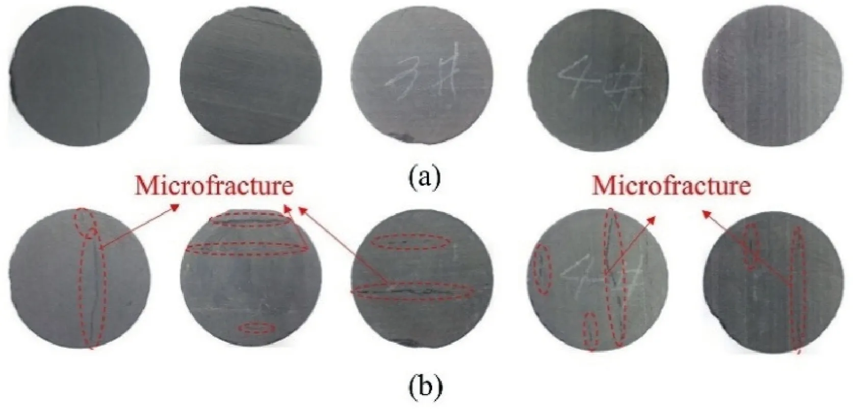
Fig.1.Comparison of shale before and after water absorption: (a) Pre-test and (b)Post-test.

Fig.2.Water absorption results from shale.

2.2.Microfracture extraction

In this study,CT experiments were performed on postabsorption shale using a Nano-CT Xradia CT instrument (Fig.3),which employs a high-resolution 3D imaging system for X-rays with a spatial resolution of 65 nm.This instrument was used to scan the core after water absorption and to analyze its microstructure and physical properties.The core sections in theXandYdirections were obtained after CT scanning(Fig.3),where black represents therock skeleton and white represents the microfractures and core pores.

Fig.3.Core slice diagram.

Based on the CT scanning results,a digital core model (Fig.4)was built.The microfractures and pores of the built digital core were imaged,where gray represents the rock skeleton,red represents the rock pore structure,and blue represents the pores and microfractures.

Fig.4.Core reconstruction.

There are some unconnected spaces in the reconstructed 3D model of shale because the extraction effect of pores and microfractures is poor (Fig.3).To simulate two-phase flow in microfractures,it is necessary to select appropriate thresholds,improve the contrast between pores and microfractures,and extract microfractures for research.

The idea of the maximum class spacing method is consistent with the characteristics of the core CT image itself,and the CT image can obtain good results when it is segmented by the maximum class spacing method.In this section,the use of the maximum class distance method for threshold segmentation is discussed.The basic idea is that suppose a set contains the gray values of all voxels in the image to be segmented,and the set of gray values is divided into two groups by threshold;when the ratio of the intra-group variance to inter-group variance of the two groups is the largest,the corresponding segmentation value is a reasonable threshold.The microfractures and pore spaces in the core can be divided into groups,and the internal differences of each group are small,but there are significant differences between the groups.When the set is divided by a reasonable division value,the ratio of the differences between the two groups to the differences within the group will reach a maximum,thus achieving the purpose of distinguishing pores from microfractures.

The fractures in core reconstruction (Fig.4) include a small number of macro-fractures,which should be distinguished from microfractures for further analysis.Macro-fractures typically have a length exceeding 0.1 m,aperture between 0.1 and 0.3 mm,and a tip angle of 0°-10°.In contrast,microfractures are much smaller and curved,with apertures ranging from 5 nm to 100 μm,and lengths typically between 10 and 1000 μm.To establish a 3D model of shale microfractures,the fractures fitting the microfracture definition with lengths of 10-1000 μm,apertures of 65-1000 nm,and relatively curved were extracted.As shown in Fig.5,in a voxel space of 400 × 400 × 800,the range of voxels corresponding to pores is approximately 100-2000 and that corresponding to microfractures is approximately 20,000.

Fig.5.Extraction result of spatial model.

3.Microfracture flow model

To consider the effect of microfracture roughness on flow,the roughness factor modified cubic law was introduced,and the gasliquid flow model in microfractures was established by applying the modified cubic law and LBM.Finally,the accuracy of the model was verified by experimentally testing its relative permeability.

3.1.Modified cubic law

Derived from a smooth plane,the cubic relationship between the single-slit flow and slit width is called the cubic law and is expressed as

whereQis the flow rate through the fracture (m3/s),bmis the mechanical width of the fracture(m),σ is the standard deviation of the height of the fracture profile,ρ is the density of the fluid(Pa s),Δhis the difference in height between the two sides of the fracture(m),Δlis the length of the fracture (m),andwis the width of the fracture (m).

As the actual microfracture surface is uneven,the height of the fracture surface constantly changes.The fracture surface follows self-affine fractal statistics,and the probability of the microfracture height satisfies the Gaussian distribution:

To consider the influence of fracture roughness on seepage,the standard deviation of the microfracture height is considered as the roughness factor and roughness correction,and the expression of the correction model is as follows:

wherefσ is the roughness factor that represents the weakening effect of the roughness characteristics of the fracture surface on the fluid flow.

The weakening effect of the rough characteristics of the fracture surface on the fluid flow can be treated as an external force term,to describe the effect of the rough feature on the flow.The LBM correction equation containing the external force term is expressed as

wherefi(x,t)is the distribution function alongeidirection,is an equilibrium state density distribution function,τ is the dimensionless relaxation time,eiis the discrete velocity(m/s),Fiis the external force term,and Δtis the time increment (s).

The external force term is expressed as (Guo et al.,2002):

wherecis the Lattice velocity (m/s),uis the macroscopic velocity(m/s),andwiis the lattice weight.

The relationship between the flow rate in modified cubic law and the macroscopic velocity in the external force term is expressed as

Substituting Eq.(3)into Eq.(6),the macroscopic velocity in Eq.(5) can be obtained as

3.2.Relaxation time and boundary conditions

The grid size of pore microfracture model in the LBM modeling was 400 × 400 × 800 voxels.The left side of the model is set as a constant pressure boundary of 40 MPa.The right boundary of the model is set as a pressure boundary of 10 MPa.

The relaxation time is the average time interval between two collisions in the lattice Boltzmann and can be expressed as (Timm et al.,2017):

where ν is the viscosity of the fluid (Pa s),andcsis the lattice velocity (m/s).

Nitrogen was used as the simulated fluid,and in this study,the actual boundary was a non-slip boundary.Therefore,the standard bounce format was used to deal with the solid-liquid boundary.It is assumed that after reaching the target node,particles in the middle of the migration process bounce back directly along the original direction of the particle injection.Microscopically,particles shot at the solid boundary were treated by steering them directly toward the three distribution functions of the wall via contact.

The distribution function bounces in the original direction in the standard bounce format and is expressed as

3.3.Model verification

3.3.1.Verification of pore distribution

Pore distribution characteristics can be described quantitatively using the pressure pump method(Wardlaw and Taylor,1976;Yuan and Swanson,1989).According to the pore size distribution test of the core after the experiment,its accuracy was verified by comparing it with the digital core established by the CT method.

In this study,the distribution of the pore size was measured using the mercury intrusion meter of the American Conta Poremaster 60 GT,which has a maximum pressure of 60,000 psi,a pore size range of 3 nm-1080 μm,and a maximum sample volume of 2 cm3.The rock microstructure was destroyed,and the data for micropores and partial mesopores were distorted under high pressure.Therefore,the microfractures and partial mesopores produced by shale after water absorption were the main test ranges.According to the experiment,the capillary pressure curve can be obtained,wherein the porosity,pore volume,pore distribution,specific surface area and pore size of the sample can be analyzed.

The pore size distribution in the model was obtained using the software ImageJ,and the pores in the model were highlighted by adjusting the appropriate threshold values.The statistical analysis function allows for the filtering of particles of a defined diameter to obtain the number of particles of different pore sizes in the model.The ratio of the number of pores with a defined diameter to the total number of pores in the model was obtained as the pore-size distribution of the model.

The results demonstrated that the pore size distribution trend of the actual core was consistent with that of the reconstructed core.The reconstructed core had a larger pore size,but it was generally in good agreement with the actual experimental sample (Fig.6).

Fig.6.Comparison between experimental and simulation results.

3.3.2.Flow model verification

Based on Darcy’s law,the relative permeability of rock samples treated with a working fluid was tested using the steady-state method,and the correctness of the model was verified,assuming that two-phase fluids are immiscible and incompressible.

When the total flow rate of the experiment was constant,gas and water phases were injected into the rock sample at a constant rate.The water saturation of the rock sample did not change when the pressure difference and the flow rate were stable.At this time,gas and water were stable in the rock sample.The effective permeability and relative permeability values can be calculated by measuring the pressure difference and flow rate of the rock samples at the entrance and exit.The relative permeability under different water saturation conditions was obtained,and the relative permeability curves were obtained by changing the proportion of fluid injection flow.

Compared with the experimental results,the relative permeabilities of the wetting phase (fracturing fluid) and non-wetting phase (nitrogen) obtained via the LBM simulation of cores treated with different working fluids are in a good agreement (Fig.7).

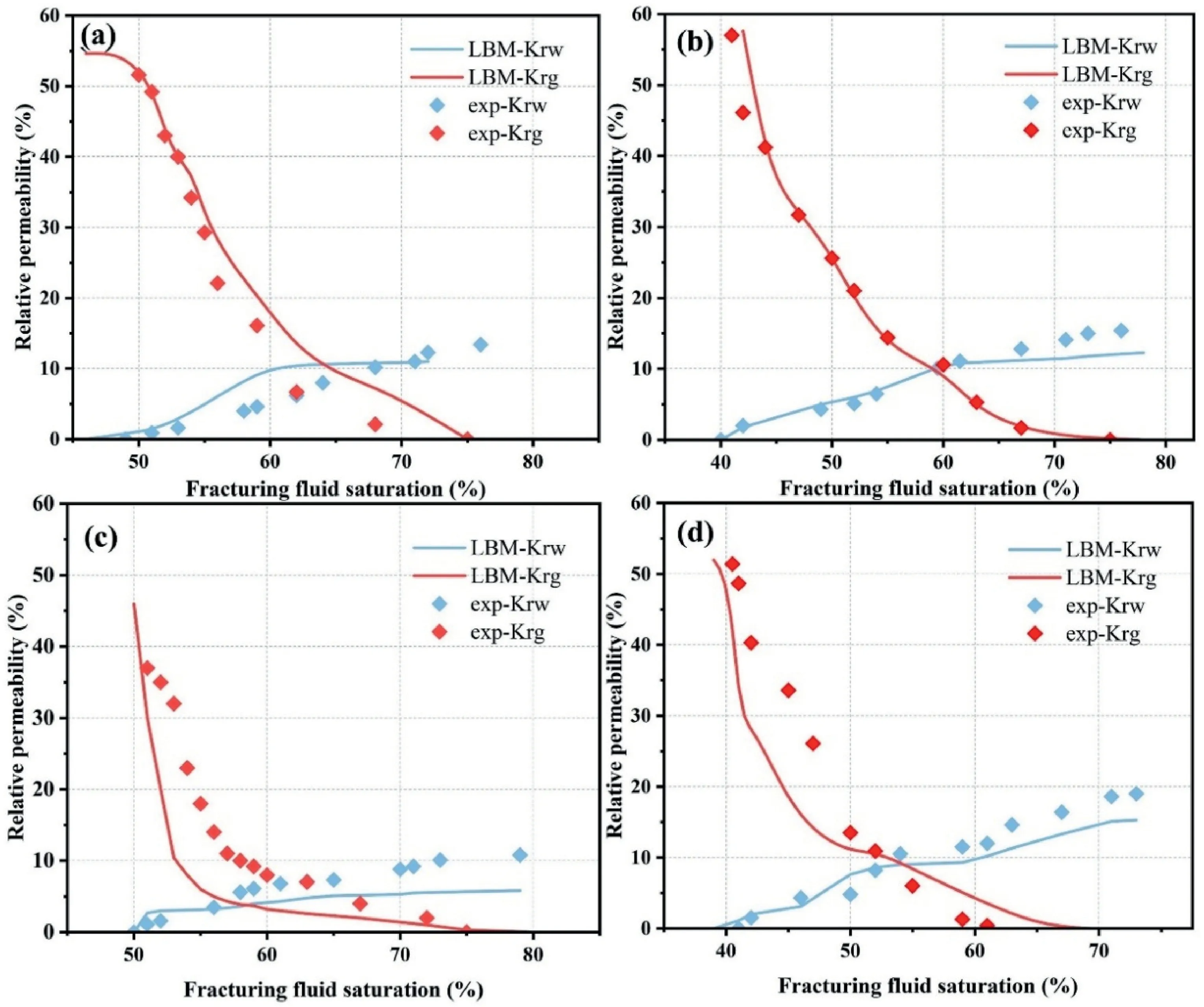
Fig.7.Relative permeability of core samples: (a) Sample 4-4,(b) Sample 8-3,(c) Sample 16-2,and (d) Sample 18-1.

4.Analysis of fluid flow characteristics in shale microfractures

4.1.Flowback characteristics of different liquids

The fluid parameters,such as the surface tension,viscosity,wettability and salinity,have different effects on the flowback.For the same microfracture physical model,the differential pressure was set to 30 MPa and the simulation time was 30 min to simulate the flow characteristics of different aqueous phase fluids of slippery water,distilled water,glue breaking solution,and 2%KCl solution in the microfracture.

The water saturation in the fracture was calculated according to the simulation,where red represents the gas.According to the comparison of water saturation in the fracture(Fig.8),the flowback capacity,from the largest to the smallest,is as follows: glue breaking solution >slippery water >2% KCl solution >distilled water.The difference in the simulation results is the comprehensive result of the differences in the wettability,surface tension,and viscosity of different liquid systems.Owing to the basic characteristics of low viscosity,high surface tension,and good wettability of distilled water,it is easier to self-absorb into the matrix and remain in the microfractures,reducing the permeability of the fractures.To increase gas production,the formula of the fracturing fluid can be adjusted from the perspectives of viscosity,surface tension,wettability improvement,and low salinity.

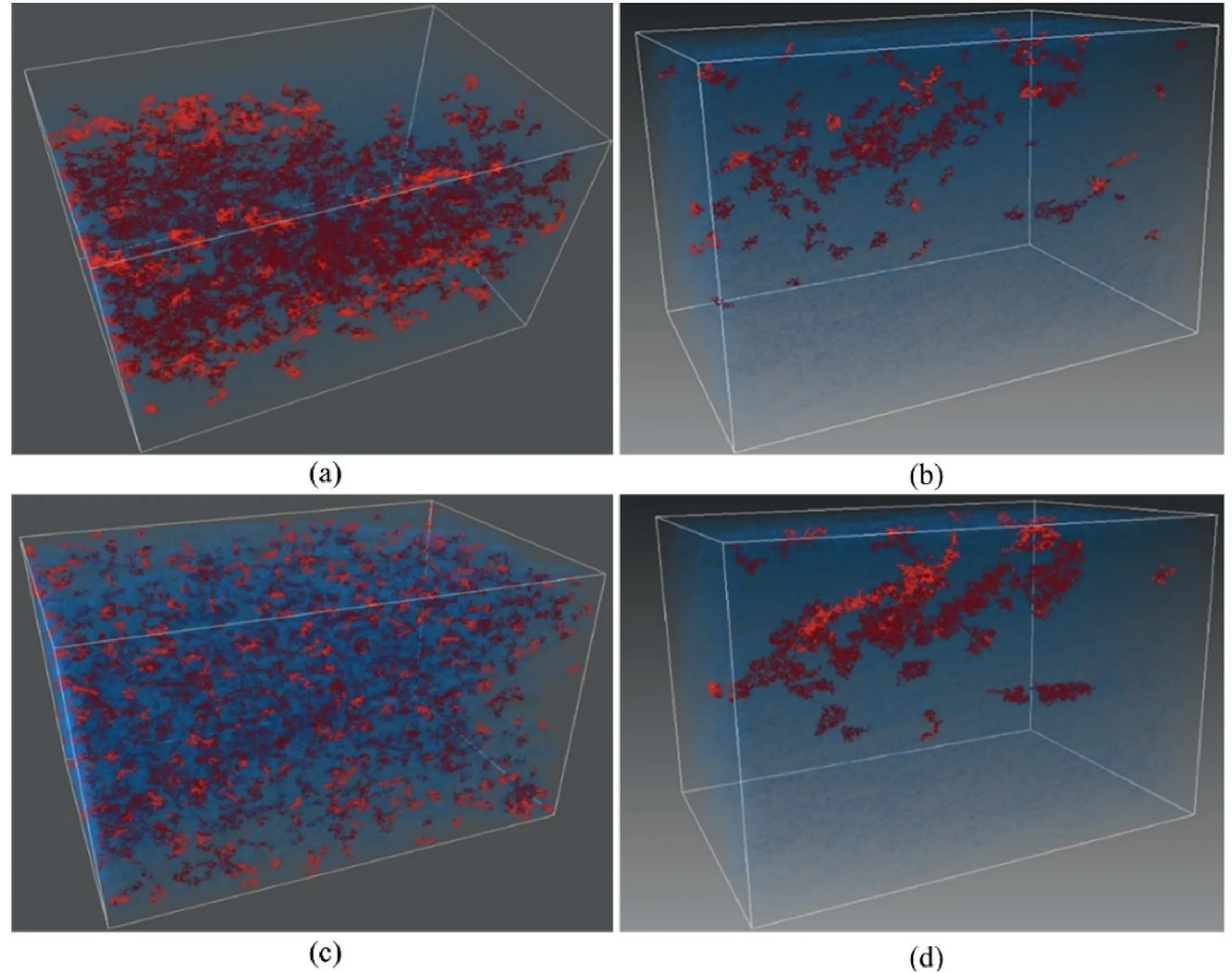
Fig.8.Simulation of different liquid flows in microfracture: (a) Slippery water,(b) Distilled water,(c) Glue breaking solution,and (d) 2% KCl solution.

4.2.Microfracture flowback characteristics

Assuming that the microfractures are filled with liquid in rock samples after self-absorption,simulations of microfracture flow were performed to investigate the characteristics of gas fracturing fluid flow at the initial stage of shale fracturing.The liquid was in the wetting phase,and the simulation was stopped after the gas phase broke through.

4.2.1.Effect of the presence of microfractures

The presence of microfractures has a significant influence on the flowback of the fracturing fluid.When microfractures are present,the fluid stored in the pore space flows through the microfractures,and in the absence of microfractures,the fluid in the pore space is too slow to be transported in the pore hole.

To clarify the mechanism of microfractures affecting fracturing fluid flowback,it is necessary to compare the flowback characteristics of the fracturing fluid in the presence of microfractures with those in the absence of microfractures.The flow patterns of gas and fracturing fluid in the microfractures were analyzed at a pressure difference of 30 MPa and a simulation time of 30 min and compared with the situation without microfractures inside the model to analyze the effect of microfractures on fluid flow,where red represents the gas phase.

The simulation results demonstrate that the fracturing fluid saturation is approximately 100% without microfractures but only 65% with microfractures.The microfractures form a continuous channel in which the gas displaces some of the fracturing fluid,whereas the fracturing fluid in the small pore cannot be displaced.This indicates that the microfractures communicate with the shale pore channels and preferentially form a continuous flow space with larger pore channels,thereby displacing a large amount of fracturing fluid from them (Fig.9).

4.2.2.Effect of microfracture spacing

The distribution of microfractures was different in different fracturing sections.Therefore,in this section,three sets of microfractures with fracture spacings of 67 μm,123 μm and 300 μm were used to simulate the two-phase flow at a pressure difference of 30 MPa.

According to the digital core model,microfractures with different spacings were extracted(Fig.10).The smaller the spacing between microfractures,the smaller the saturation of the water phase after the simulation.However,the influence of the overall microfracture spacing is not obvious (Fig.11).

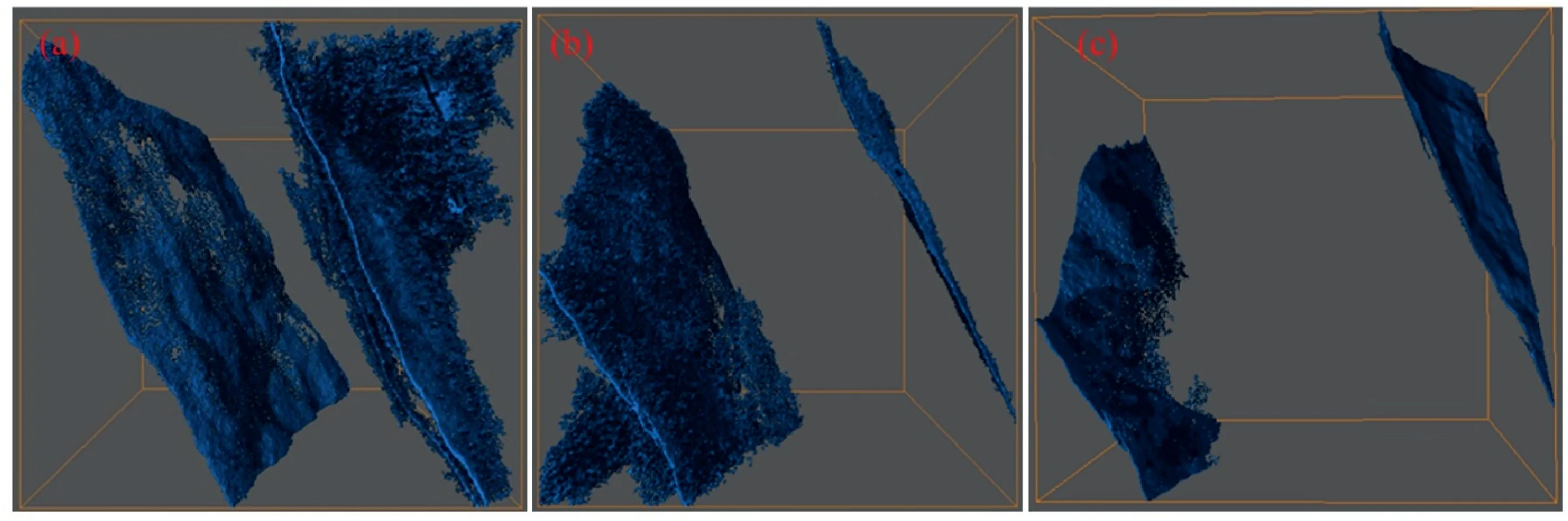
Fig.10.Fracture space model extraction results: (a) Microfracture 1,(b) Microfracture 2,and (c) Microfracture 3.

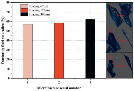
Fig.11.Simulation results of microfractures with different spacings.

4.2.3.Effect of tortuosity of microfractures

Actual shale fracture flow channels or capillaries are curved and are usually described by the tortuosity (Fig.12):

Fig.12.Schematic diagram of the tortuosity of the streamline.

whereTis the tortuosity(%),Ltis the actual length of the fluid path(m),andLis the straight-line length or characteristic length in the direction of the pressure gradient (m).

Jacques and Maurice (1989) used an experimental method to determine the tortuosity by constructing a fixed model of porous media,combining the Darcy’s law and the Poiseuille formula to obtain the permeability of porous media,and then back-calculating the tortuosity.Yu (2005) derived an equation for the average tortuosity using the fractal dimension method,which is expressed as

where φ is the porosity (%).

In this study,microfractures with different degrees of tortuosity were extracted from the internal structure of the shale,and based on the results obtained,the improved Dijkstra algorithm was used to determine the shortest flow length in the microfracture.Then,the ratio of the straight-line distance between the two ends of the fracture was used to determine the tortuosity of each microfracture.

The basic idea of the improved Dijkstra’s algorithm is as follows(He,2022):(1)Read the data and initialize it toS={sp};(2)Find the nodeiwith the shortest distance fromsp,and substitute it intoS;(3)Find the nodeithat can be reached once in the starting pointU,and modify the shortest distance value.IfD(j)＞D(i)+d(i,j),then update it toD(j)=D(i)+d(i,j),and substituteiinto pre(j),jandS;(4)Repeat Steps(2)and(3)until all the data are read;(5)Sis the set of shortest path nodes,andDis the set of path lengths.The calculated microfracture tortuosity was compared with the experimental results and the results of the tortuosity equations derived by Yu (2005).The maximum error is 7.8%,indicating that the tortuosity can be reliably calculated using the Dijkstra algorithm(Table 2).

Table 2Tortuosities of different microfractures.

The fluids were gas and slippery water with a differential pressure of 30 MPa.The gas-fracturing fluid two-phase flow process in the four microfractures was simulated (Fig.13).The simulation results demonstrate that the saturation of the fracturing fluid in the microfractures increases with an increase in the tortuosity.The greater the tortuosity,the worse the flow capacity of the fluidin the microfractures and microfracture,and the higher the saturation coefficient of the liquid phase (Fig.14).

Fig.13.Microfractures of different tortuosities.

Fig.14.Simulation results of microfractures with different tortuosities.

4.2.4.Effect of microfracture volume

To investigate the effect of microfracture volume on fracturing fluid flowback,a two-phase flow simulation of microfractures with different volumes was carried out,where the type of fracturing fluid in the model was slippery water(Fig.15).It is assumed that in this model,the water phase intrudes into and microfractures.In the simulation process,a continuous channel is formed in the microfracture after the gas invades,which can displace the fracturing fluid in the fracture.However,the fracturing fluid in the small channels inside the shale could not be displaced.The larger the volume and fracture area of the shale seam network fracturing transformation,the more difficult the fluid flow.

Fig.15.Simulation results of different shale internal space flow: (a) Microfracture of small volume,(b) Microfracture of medium volume,and (c) Microfracture of large volume.

4.3.Flowback characteristics under different pressure differences

To study the effect of the production pressure difference on the fracturing fluid flowback rate of shale and determine a reasonable flowback system,the two-phase flow simulations of microfractures with various production pressure differences (10 MPa,20 MPa,30 MPa,40 MPa) were carried out.The simulation results are as follows,where red represents the gas phase (Fig.16).

Fig.16.Flow simulation results corresponding to different production pressure differences: (a) 10 MPa,(b) 20 MPa,(c) 30 MPa,and (d) 40 MPa.

Under low differential pressure,the resistance of the gas to the fracturing fluid was small.The liquid-carrying capacity of the gas is poor,causing a large fracturing fluid saturation in microfracture,which demonstrates that the liquid remains in the microfracture under the condition of a low pressure difference.However,under the condition of a high pressure difference,the liquid-carrying capacity of the gas for the fracturing fluid becomes stronger,and the saturation of the liquid phase in the fracture decreases.However,under the action of the surface tension between the water phase,rock wall,and capillary force,the liquid phase remains in the rock wall and pore throats.By contrast,with an increase in the pressure difference,there was no noticeable decrease in water saturation (Fig.17).

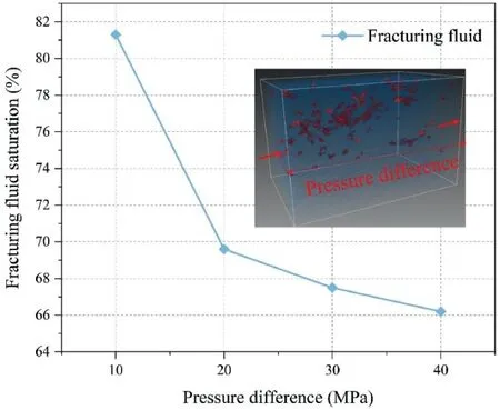
Fig.17.Liquid phase saturation distribution at different pressure differences.

5.Conclusions

Based on the CT reconstruction of the core pore microfracture model,a rough factor modified cubic law was introduced and combined with LBM to establish a model for the flowback of fracturing fluid in shale pores and microfractures.The conclusions are drawn as follows:

(1) The flowback model of the reconstructed microfractures was established,and the flowback law of shale in the initial stage of flowback was investigated.At the initial stage of flowback,the fracturing fluid entered the shale pores and replaced the gas in them,and the replaced gas entered the microfracture to form a gas-water two-phase flow with the fracturing fluid.

(2) According to the flowback simulations of different fracturing fluids,the saturation of the glue breaking fluid in the core was the lowest.This indicates that the displaced amount of glue breaking fluid is the largest,and the flowback rate of the glue breaking fluid is the highest,providing a reference for the selection of fracturing fluid types and formulations in the field.

(3) This study applied an improved Dijkstra’s algorithm to determine the shortest streamline length in a microfracture and then compared it to the straight-line distance between the two ends of the fracture to obtain the tortuosity of the fracture.This algorithm considered the real internal 3D structure of the core as the model and did not rely on empirical formulae to calculate the tortuosity,which significantly improved the accuracy of the solution.The effect of microfracture tortuosity on the fracture fluid flowback was then analyzed;the greater the tortuosity,the more curved the streamline,and the poorer the flow capacity of the fracture fluid in the microfracture.

(4) By simulating the flowback under different internal rock structures,the flowback characteristics were discovered.The gas formed a continuous channel in the microfracture,displacing some fracturing fluids.

(5) The resistance of the gas to the fracturing fluid was small,and the liquid-carrying capacity of the gas was poor under the condition of a low pressure difference.Thus,the liquid in the microfracture could not be discharged together with the gas.However,the carrying capacity of the gas to the fracturing fluid increased and the saturation of the liquid phase in microfractures decreased under the condition of a high pressure difference.

Declaration of competing interest

The authors declare that they have no known competing financial interests or personal relationships that could have appeared to influence the work reported in this paper.

Acknowledgments

This study was supported by the National Natural Science Foundation of China (Grant No.52022087).It was prepared under the auspices of the State Key Laboratory of Oil and Gas Reservoir Geology and Exploitation at the Southwest Petroleum University.