Influence of ground effect on flow field structure and aerodynamic noise of high-speed trains

XiaomingTAN,LinliGONG,XiaohongZHANG,ZhigangYANG

Research Article

Influence of ground effect on flow field structure and aerodynamic noise of high-speed trains

1Key Laboratory of Intelligent Manufacturing and Service Performance Optimization of Laser and Grinding in Mechanical Industry, Hunan Institute of Science and Technology, Yueyang 414000, China2Key Laboratory of Traffic Safety on Track (Central South University), Ministry of Education, School of Traffic & Transportation Engineering, Central South University, Changsha 410075, China

The simulation of the ground effect has always been a technical difficulty in wind tunnel tests of high-speed trains. In this paper, large eddy simulation and the curl acoustic integral equation were used to simulate the flow-acoustic field results of high-speed trains under four ground simulation systems (GSSs): “moving ground+rotating wheel”, “stationary ground+rotating wheel”, “moving ground+stationary wheel”, and “stationary ground+stationary wheel”. By comparing the fluid-acoustic field results of the four GSSs, the influence laws of different GSSs on the flow field structure, aero-acoustic source, and far-field radiation noise characteristics were investigated, providing guidance for the acoustic wind tunnel testing of high-speed trains. The calculation results of the aerodynamic noise of a 350 km/h high-speed train show that the moving ground and rotating wheel affect mainly the aero-acoustic performance under the train bottom. The influence of the rotating wheel on the equivalent sound source power of the whole vehicle was not more than 5%, but that of the moving ground slip was more than 15%. The average influence of the rotating wheel on the sound pressure level radiated by the whole vehicle was 0.3 dBA, while that of the moving ground was 1.8 dBA.

High-speed train; Aero-acoustics; Flow field structure; Large eddy simulation; Moving ground condition; Rotating wheel

1 Introduction

As high-speed ground transportation vehicles, high-speed trains inevitably encounter ground effect problems, that is, disturbance caused by the ground boundary layer to the structure of the train bottom flow fields. The accuracy of simulation of the ground effect phenomenon has a great effect on the accuracy of predictions of high-speed train aerodynamics and aerodynamic noise.

Prediction models are widely used at present to understand the nature of railway ground waves and their associated characteristics (Kouroussis et al., 2021). Using boundary layer correction theory to correct the simulation results of aerodynamic force and aerodynamic noise of 3D complex structures such as high-speed trains is difficult. The main techniques available to eliminate the negative effects of ground effect in wind tunnel tests include the moving ground method, tangent blow-suction method, and suction method. The moving ground method is the most satisfactory for its capacity to simulate the relative motion between the train, ground, and air. Using the moving ground method, Tyll et al. (1996) estimated the aerodynamic drag coefficients of maglev to be 0.24 with moving rails and 0.17 without rails. Moreover, they pointed out that a moving track is very important to the accuracy of aerodynamic testing of a maglev train. Yi et al. (1997) investigated the ground effect of a high-speed train using the suction method. They showed that the elimination of the boundary layer can significantly increase the aerodynamic drag force coefficient, the increment of which depends on the shape of the train bottom. By comparing the test results from the tangent blow-suction method and the moving ground method, Kwon et al. (2001) concluded that the tangential blowing method was an effective substitute for the moving ground method for testing aerodynamics.

Xia et al. (2016) compared train wind simulation results between the stationary ground and the moving ground conditions and concluded that the stationary ground result was larger than that of the moving ground. In the following year, they constructed seven ground simulation systems (GSSs) and pointed out that the elimination of the boundary layer can significantly increase the aerodynamic drag coefficient, and that elevation of the model cannot effectively eliminate the adverse effects of the ground effect (Xia et al., 2017). Zhang et al. (2016) numerically simulated the train aerodynamic simulation results of three GSSs: "stationary ground+stationary wheel", "moving ground+stationary wheel", and "moving ground+rotating wheel", and concluded that the moving ground could significantly increase the aerodynamic drag coefficient, while the rotating wheel could not. Paz et al. (2017) evaluated the influence of sleepers on the aerodynamic drag coefficient on the ground effect through the dynamic layering method. They found that the existence of sleepers had a great impact on the aerodynamic performance of the whole train, increasing the aerodynamic drag coefficient by about 15%, but had little impact on the lift coefficient. Zhu et al. (2017) numerically calculated the aerodynamic noise radiated by a wheelset of two GSS conditions: moving ground and no ground. They found that the result of moving ground was about 7 dB higher than that of no ground. The simulation results of aerodynamic noise of high-speed trains by Liu et al. (2013) showed that the result of moving ground was 4‍–‍6 dBA larger than that of stationary ground. Wen et al. (2019) found that the existence of bogies on the bottom of the train, especially the last bogie, not only enhanced the wake flow but also introduced large perturbances into the wake flow. The bogie effects were revealed through a systematic comparison of flow structures, slipstream characteristics, and aerodynamic forces between two generic train configurations (Shibo et al., 2018).

To sum up, we now have a more comprehensive and accurate understanding of how the ground effect influences the prediction accuracy of aerodynamic force, but how the ground effect influences the prediction accuracy of aerodynamic noise is still unclear. The reason is that the current methods of eliminating the ground boundary layer cannot account for either changes in the fluctuating flow field at the train bottom or the generation of new noise. The ground is assumed to be stationary in current acoustic wind tunnel tests, and it is impossible to explore the influence laws of different GSSs on aero-acoustic tests. On the other hand, the current geometric models for numerical simulation are simplified. In this study, we constructed numerical models of four GSSs to explore the influence laws of different GSSs on the flow field structure and aerodynamic noise, and to provide guidance for the acoustic wind tunnel testing of high-speed trains.

2 Numerical simulation model

The geometric model was a 1/8-scale high-speed train model with three carriages, bogies and without a pantograph (Tan et al., 2018). The model was 7960 mm long, 4080 mm high, and 3360 mm wide. The geometric model was divided into 32 parts, i.e., Components #1‍–‍#32. The naming rules of the first 20 parts are shown in Fig. S1 of the electronic supplementary materials (ESM), and the last 12 parts correspond to the 12 wheelsets. From upstream to downstream, the wheelset was named sequentially from Component #21. For example, Component #21 corresponds to the front wheelset of Bogie 1, and Component #22 corresponds to the back wheelset of Bogie 1.

The simulated incoming velocity was 350 km/h. The surface of the train model, excluding the 12 wheelsets, was set as a non-slip boundary condition with friction. All wheelsets were set to a speed of 1817.2 or 0 rad/s. The wheel speed is derived from Section S1 of the ESM. The ground moving velocity was 350 or 0 km/h. These could be combined freely to form four GSSs: "moving ground+rotating wheel", "stationary ground+rotating wheel", "moving ground+stationary wheel", and "stationary ground+stationary wheel". For the convenience of discussion, they were named Case 1, Case 2, Case 3, and Case 4, respectively.

We used the Ansys Fluent software from the Wuxi Computing Centre (China) to carry out numerical simulations of the aerodynamic noise of the high-speed train. The unsteady calculation time step was 5×10-5s, and iterated 30 steps in each time step. A total of 10000 time steps were calculated. The computation of the first 2500 time steps was to ensure full development of the turbulence flow field, and that of the remaining 7500 time steps was to extract the noise source information. Sound source data in each time step were stored, with a time span of 0.375 s and a frequency resolution of 2.7 Hz. The number of body grids was about 110 million.

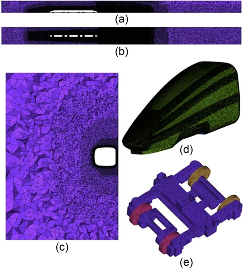
Fig. 1 Grid distribution: (a) longitudinal symmetry plane; (b) on the same elevation as the tip of the nose; (c) a cross section of the tail-flow type shoulder; (d) streamlined area; (e) bogie

3 Difference analysis of flow field structure characteristics

Through the three physical quantities of velocity amplitude, vorticity amplitude, andvalue, the differences among the four GSSs in terms of the flow field structure around the train were revealed. For convenience of description, Fig. 2 shows all sections in this study. Section a is a-equivalent plane running through the calculation domain and the wheel pair, with avalue of 93 mm. Section b is theiso-surface penetrating the calculation domain, with avalue of 50 mm. Line 1 runs along thedirection and penetrates the calculation region, with avalue of 93 mm and avalue of 12.5 mm.

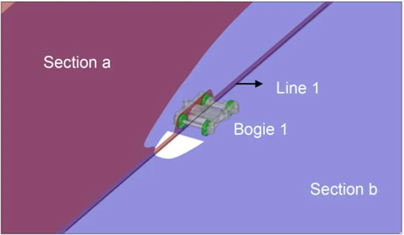
Fig. 2 Sketch map of the section

3.1 Flow velocity magnitude

From Figs. 3 and 4, the influence of the four GSSs on the spatial distribution of the velocity amplitude around the high-speed train can be obtained. The four cases had no influence on the velocity amplitude distribution in Region I, the upper part of the train. In Region II, near the nose of the head car, whether the wheel was rotating or not had little effect on the form of the stagnation zone, and the volume of the stagnation zone caused by "stationary ground" was larger than that caused by "moving ground". In Region III, the area from the discharger of the head car to Bogie 1, the length of the acceleration zone under the "moving ground" condition was larger than that under the "stationary ground" condition. When the wheel was rotating, the velocity amplitude inside the cavity was increased. In Region IV, the area from beneath Bogie 2 to Bogie 3, the velocity amplitude under "moving ground" was larger than that under "stationary ground", and so was the velocity amplitude inside the cavity. In Region V, the wake area near the discharger of the tail car, the low-speed zone in "moving ground", was smaller than that in "stationary ground". Nevertheless, whether the wheel was rotating or not hardly affected the velocity amplitude distribution in this region. Note that the velocity amplitude distribution of the ground area under "stationary ground" was closely related to the grid scale and ground boundary layer effect.

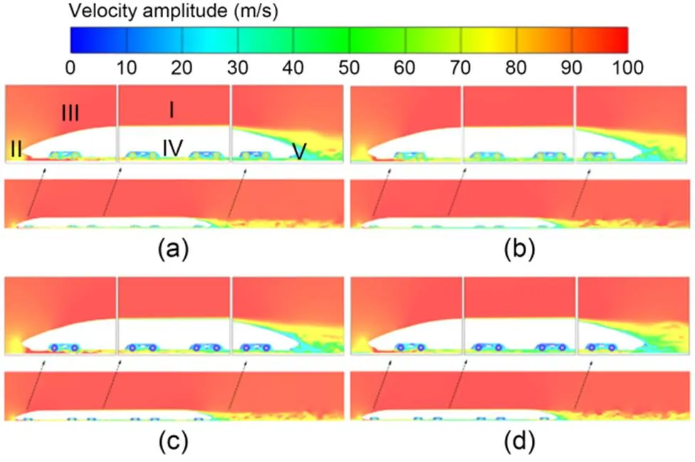
Fig. 3 Instantaneous velocity amplitude contour of Section a: (a) Case 1; (b) Case 2; (c) Case 3; (d) Case 4

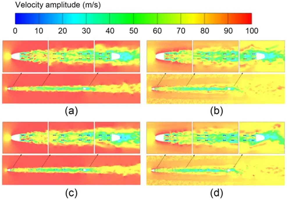
Fig. 4 Instantaneous velocity amplitude contour of Section b: (a) Case 1; (b) Case 2; (c) Case 3; (d) Case 4

To quantitatively analyze the velocity amplitude distribution formed in the four GSSs, Table 1 shows the mean value of the velocity amplitude of Line 1.

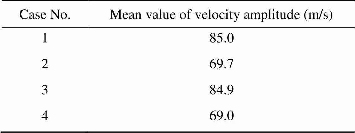
Table 1 Mean value of the velocity amplitude

Whether the wheel was rotating or not hardly affected the velocity amplitude of Line 1, while the velocity amplitude of Line 1 on moving ground was 23% larger than that on stationary ground (Table 1).

3.2 Vorticity magnitude

From Figs. 5 and 6, we can obtain the effects of the four GSSs on the spatial distribution of vorticity amplitude around high-speed trains. The four cases had no effect on the vorticity amplitude distribution in Region I, the upper part of the train. In Region II, near the nose of the head car, the state of the wheel had little effect on the vorticity distribution. However, the vorticity distribution on "stationary ground" was uneven, but relatively uniform on "moving ground". In Region III, the area from the discharger of the head car to Bogie 1, the "moving ground" decreased the vorticity amplitude between the train and the ballast compared with the "stationary ground". In Region IV, the area from beneath Bogie 2 to Bogie 3, whether the ground was moving or not had little effect on the vorticity distribution in that region. In Region V, the wake area near the discharger of the tail car, both "stationary ground" and "moving ground" conditions could form strong vorticity separation flow at the shoulder of the tail car streamline and form a strong vortex mixing flow in the tail car cowcatcher bottom and downstream area. But the separation flow formed in the "stationary ground" condition was closer to the streamlined car body downstream, and the mixed flow formed by "stationary ground" showed large-scale rotating flow intensity and strong swing strength on both sides. Besides, whether the wheel was rotating or not hardly affected the vorticity distribution of this region. Note that the amplitude distribution of vorticity was closely related to the grid scale and the boundary layer effect. The larger the grid scale, i.‍e, the further away from the high-speed train area, the more uneven the cloud map of vorticity amplitude distribution, and the larger the voracity amplitude. Nonetheless, these phenomena did not appear under the "moving ground" condition.

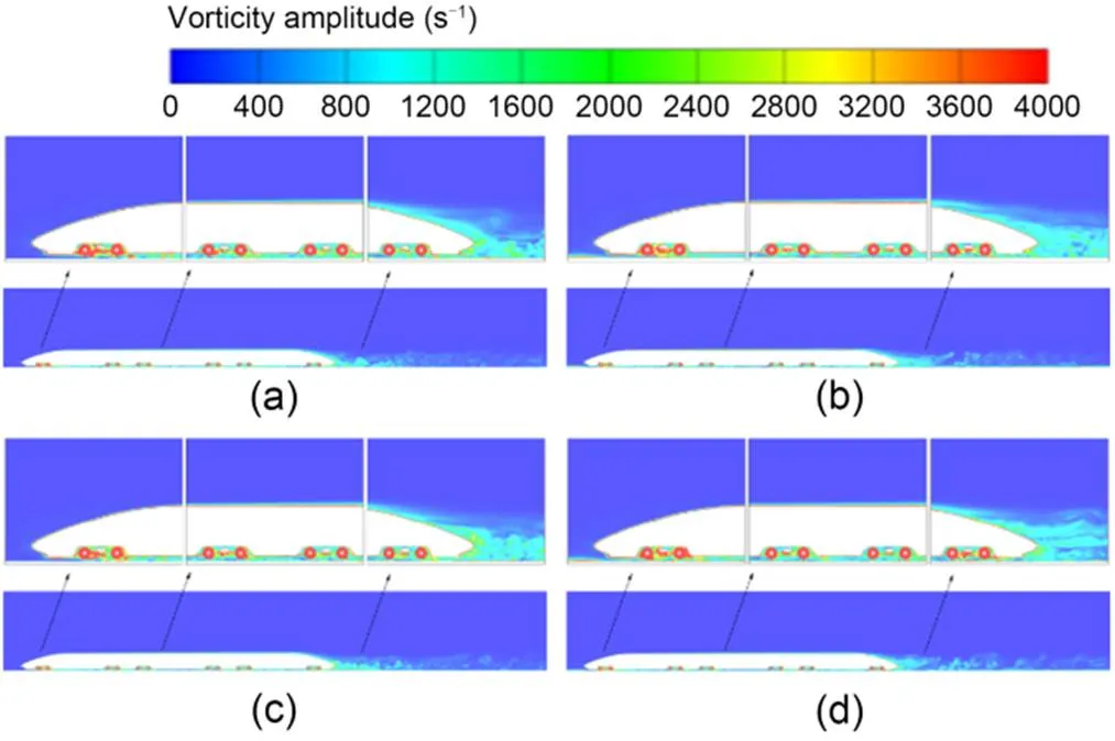
Fig. 5 Instantaneous contour plot of vorticity amplitude at Section a: (a) Case 1; (b) Case 2; (c) Case 3; (d) Case 4

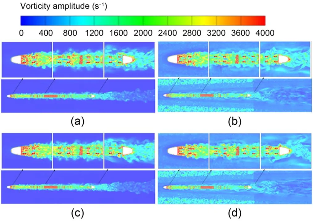
Fig. 6 Instantaneous contour plot of vorticity amplitude at Section b: (a) Case 1; (b) Case 2; (c) Case 3; (d) Case 4

The vorticity amplitude distribution formed in the four GSSs was analyzed. Table 2 shows the mean value of the vorticity amplitude of Line 1. Table 2 shows that whether the wheel was rotating or not hardly affected the vorticity amplitude of Line 1, while the vorticity amplitude of Line 1 on stationary ground was up to 631.3% larger than that on moving ground.

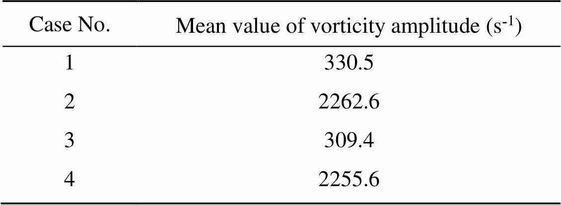
Table 2 Mean value of the vorticity amplitude

3.3 Q value

As shown in Figs. 7 and 8, we can observe the influence of the four GSSs on the spatial distribution of the scale/strength of the vortex structure around the high-speed train. The four cases had no influence on the spatial distribution of the scale/strength of vortex structure in Region I, the upper part of the train. In Region II, near the nose of the head car, the four GSSs hardly affected the vortex structure scale/strength spatial distribution. In Region III, the area from the discharger of the head car to Bogie 1, the vortex structure formed in the "moving ground" condition was larger than that in the "stationary ground" condition, and the moving speed of the vortex structure was faster along both sides. Compared with the "stationary wheel" case, the "rotating wheel" case slightly increased the scale and strength of the vortex structure inside the cavity, but decreased the number of the vortexes inside the cavity and propagated a larger group of vortexes downstream. In Region IV, the area from beneath Bogie 2 to Bogie 3, the scale of the vortex structure under "moving ground" was larger than that under "stationary ground". There was also a stronger tendency of the vortex to move to both sides. In Region V, the wake area near the cowcatcher of the tail car, the vortex group structure rotated around the center in the "stationary ground" condition and formed a larger vortex structure on the upper part of the tail streamline than in the "moving ground" condition. However, whether the wheel was rotating or not hardly affected the formation/revolution of the vortex structure in this region. Note that the "moving ground" conveyed the vortex group structure formed in the wake region farther downstream than did the "stationary ground" condition.

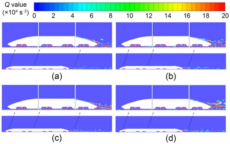
Fig. 7 Instantaneous contour plot of Q value at Section a: (a) Case 1; (b) Case 2; (c) Case 3; (d) Case 4

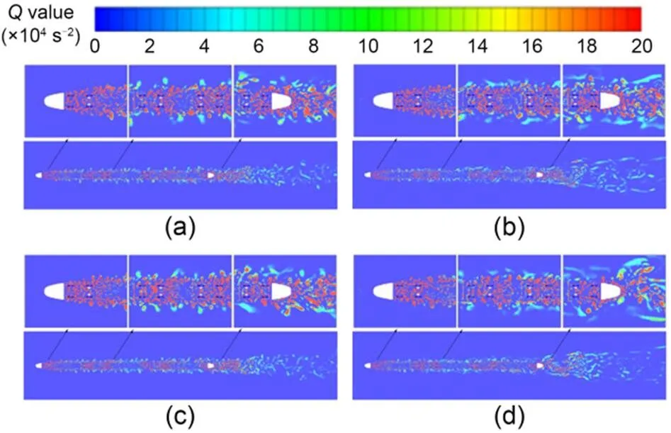
Fig. 8 Instantaneous contour plot of Q value at Section b: (a) Case 1; (b) Case 2; (c) Case 3; (d) Case 4

In summary, compared with "stationary ground", the "moving ground" cases increased the velocity amplitude of the flow between the train and the ballast, the scale of the vortex structure, and the vortex groups transporting downstream. Furthermore, it enhanced the tendency of the vortex group under the train to move to the sides. The "rotating wheel" increased the velocity amplitude inside the cavity, the vortex amplitude and structure scale/strength, and the scale of the vortex group conveyed downstream. Also, it enhanced the shear flow release strength of the bogie guides and decreased the amount of vortex groups inside the cavity. Note that the distributions of velocity and vorticity amplitude near the ground in the "stationary ground" case were linked to the grid scale and ground boundary layer effect. However, those phenomena did not appear in the "moving ground" condition. In addition, compared with the "moving ground" condition, the vortex structure rotating around the center in the wake mixing zone under the "stationary ground" condition was more identifiable, and a large scale of vortex structure was formed above the tail streamline.

The reasons for the difference in the simulated ground flow field between the four GSSs are as follows. A boundary layer forms in the "stationary ground" and becomes thicker along the train, while the velocity inside the boundary layer is lower than the main flow, thereby preventing more air from flowing into the head car bottom and out of the tail car. Therefore, air accumulates at the head car upstream and the tail car downstream. The velocity gradient of the boundary layer is large resulting in the large vortex amplitude. But the vortex amplitude of the "moving ground" is small and conveys a strong vortex flow generated by the bogie cabin to the downstream. Therefore, the velocity amplitude of the upstream train bottom space under the "moving ground" is small, but the velocity amplitude of the downstream train bottom space is almost the same as that of the "stationary ground".

Among the four GSSs, the "moving ground+rotating wheel" had the closest emulation of the true flow field, followed by the "moving ground+stationary wheel", while the other two GSSs hardly met the requirements for refined simulation of high-speed train aerodynamic noise.

4 Aerodynamic noise source

whereis the fluctuating pressure on the high-speed train, Pa;is the physical quantity of the Fourier transform for, Pa;is the frequency, Hz;is the fluctuating force, N;is the area of the noise source, m2; the symbol ′ represents the time derivative.

4.1 Intensity characteristics

The root mean square of the high-speed train surface fluctuating pressure change rate was defined as a function by

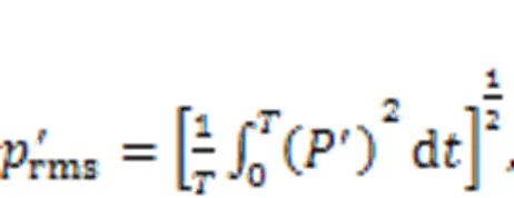
whereis the total calculation time.

Eq. (3) can be used to characterize the average effect of sound source intensity during the sampling time. Fig. 9 shows the dipole noise source intensity distribution cloud map of the train in each of the four GSSs.

Fig. 9 shows that the strength distribution law of the vehicle dipole noise source was consistent in the four GSSs. For instance, the areas with strong dipole sources included the lower sides of each bogie cabin and the bottom of the headstock and the bogies. The strength of the dipole sources on Bogie 1 was larger than that on the other bogies. However, there was little difference in the magnitude of the train body dipole noise source intensity calculated by the four GSSs. To the train bottom downstream of the head car cowcatcher, whether the wheel was rotating or not hardly influenced the dipole noise source distribution in that region, and the area of strong dipole noise source distribution under the "moving ground" was significantly larger than that under the "stationary ground". With regard to the six-bogie region, the strong dipole noise source distribution area was larger when the wheel was rotating. For the five-bogie region upstream, the area of strong dipole noise source distribution under the "moving ground" was significantly larger than that under the "stationary ground". However, at the six-bogie domains, it was just the opposite. To quantitatively analyze the dipole noise sources calculated by the four GSSs, since the flow field restored by Case 1 was the most realistic, we counted the sound power of the other three GSSs based on the equivalent sound power of each component or the whole train calculated by Case 1. The component number is in Fig. S1 of the ESM.

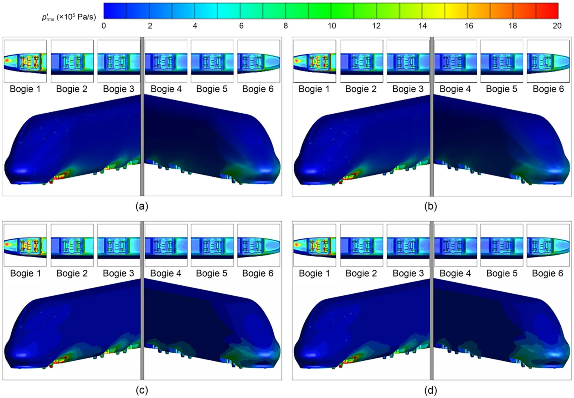
Fig. 9 Distribution cloud maps of on the surface of the train: (a) Case 1; (b) Case 2; (c) Case 3; (d) Case 4

4.2 Frequency characteristics

The effects of the four GSSs on aerodynamic noise sources were discussed above in terms of aerodynamic noise source strength. We focused only on the details of the effects of the four cases on the whole car, the bottom of the head car streamlined, the bottom of the tail car streamlined, Bogie 1, Bogie 6, and the upper part of the tail car streamlined from the sound source frequency characteristics.

For the components discussed above and the whole car, we calculated the relative percentages of the other three GSSs of the sound power equivalent to Case 1 within the corresponding frequency range based on the equivalent sound power within every frequency band (1/3 octave) (Fig. 10).

With regard to the equivalent sound power of the whole car, the result calculated by Case 3 at all frequency bands was almost the same as that of Case 1, showing a maximum difference value of 1.0 dB with the corresponding frequency band center of 40 Hz. At the frequency range of [125, 10000] Hz, the results of Case 2 and Case 4 were slightly smaller than that of Case 1, with a maximum difference of 1.9 dB with the corresponding frequency band center of 800 Hz. In the range of [20, 100] Hz, the calculation results of Case 2 and Case 4 were bigger than that of Case 1. The biggest difference was 3.2 dB and the corresponding frequency band center frequency was 50 Hz. Fig. 11 shows the percentage of the equivalent sound power result calculated by Case 2, Case 3, and Case 4 at 50 Hz relative to Case 1. The equivalent sound power at 50 Hz calculated by Case 2 and Case 4 apparently differed from that of Case 1 in the upper part of the middle car, the upper part of windshield 2, the upper part of the tail carriage and the tail car streamlined, the bottom of windshield 2, the bottom of the tail carriage and the tail car streamlined, and Bogies 4 to 6 and their wheel pairs at the downstream of the head car.

As shown in Fig. 10, the equivalent sound power of the head car streamlined bottom calculated by Case 3 was almost the same as that of Case 1 in most of the frequency bands, especially in the high-frequency range, but differed greatly in several low-frequency bands. For example, in the frequency band with a center frequency of 20 Hz the difference was 3.5 dB. The results of Case 2 and Case 4 were smaller than that of Case 1 in all frequency bands and the maximum difference was about 2.4 dB with the frequency band center frequency being 12.5 Hz.

The equivalent sound power of the tail car streamlined bottom calculated by Case 3 was almost the same as that of Case 1 in most frequency bands, but differed greatly in several low-frequency bands. For example, when the frequency band center frequency was 40 Hz the difference was up to 2.4 dB. In the frequency range where the center frequency was 12.5 Hz, the results of Case 2 and Case 4 were about 2.8 and 1.0 dB smaller than that of Case 1, respectively. At other frequency ranges, the results of Case 2 and Case 4 were bigger than that of Case 1, with a maximum of about 5.8 dB and a corresponding center frequency of 20 Hz.

The equivalent sound power of Bogie 6 calculated by Case 3 was almost the same as that of Case 1 in most frequency bands, but the results were variable in several low-frequency bands. For instance, the difference was 1.8 dB when the center frequency was 16 Hz. In most frequency bands, the results of Case 2 and Case 4 were apparently larger than that of Case 1. The largest difference was about 5.3 dB with the corresponding center frequency being 20 Hz. The result of Case 2 was slightly smaller than that of Case 1 only when the frequency band center frequency was 12.5 Hz.

In general, whether the wheel was rotating and whether the ground was moving affected the equivalent sound power mainly in the frequency range below 100 Hz. Whether the ground was moving had a more significant influence on the equivalent sound power than whether the wheel was rotating. In most frequency bands, the equivalent sound power of the head car downstream calculated by the "stationary ground" was larger than that of the "moving ground", while the components in the head car calculated by the "stationary ground" were smaller than those of the "moving ground". We adopted the same method to analyze the percentage of the equivalent sound source, and the results are shown in Fig. S2.

5 Far field radiation noise

Combined with the mirror imaging principle, the Curl acoustic integral equation can be used to calculate the far field radiation noise considering the ground effect. The calculation process is given in Section S2 of the ESM.

To study the characteristics of high-speed train radiated noise, we set 16 measuring points every 5 m along the train. These points were 25 m from the train's central axis and 3.5 m above the ground. The first point was located in the 2.5 m-position downstream of the nose of the head car. The last point was located in the 2.5 m-position upstream of the nose of the tail car. The locations of these points are shown in Fig. 12. Considering the ground reflection, we set another 16 points which were symmetric about the ground according to the specular reflection principle.

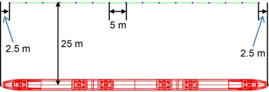
Fig. 12 Locations of the measuring points

5.1 Intensity characteristics

To study the aerodynamic noise sound pressure level (SPL), we compared the measuring point test results of the four GSSs (Fig. 13a). The difference distribution curve of whether the wheel was rotating or not is shown in Fig. 13b, and the curve of "Case 3-Case 1" represents the difference distribution curve of whether the wheel was rotating or not in the "moving ground" condition. Fig. 13c gives the difference distribution curve of whether the ground was moving or not, in which the curve marked with "Case 1-Case 2" represents the difference distribution curve in the "rotating wheel" condition and the curve "Case 3‍-‍Case 4" represents the difference distribution curve in the "stationary wheel" condition.

Fig. 13 shows that the distribution of aerodynamic noise sound pressure levels calculated by the four GSSs was consistent. But the aerodynamic noise pressure level results of the four GSSs apparently differed in their simulation values. Compared with the "stationary wheel", the result of the "rotating wheel" was smaller in the upstream, while the result tested by the downstream points was the opposite. The mean difference value of whether the wheel was rotating or not at 16 measuring points was 0.3 dBA. Compared with "stationary ground", the result for the "moving ground" of each point was larger, especially the points in the upstream, while in the downstream the difference was smaller. The average difference between whether the ground was moving or not at the 16 points was 1.8 dBA. Whether the ground was moving or not had a more significant influence on the aerodynamic noise sound pressure level radiated by the whole train.

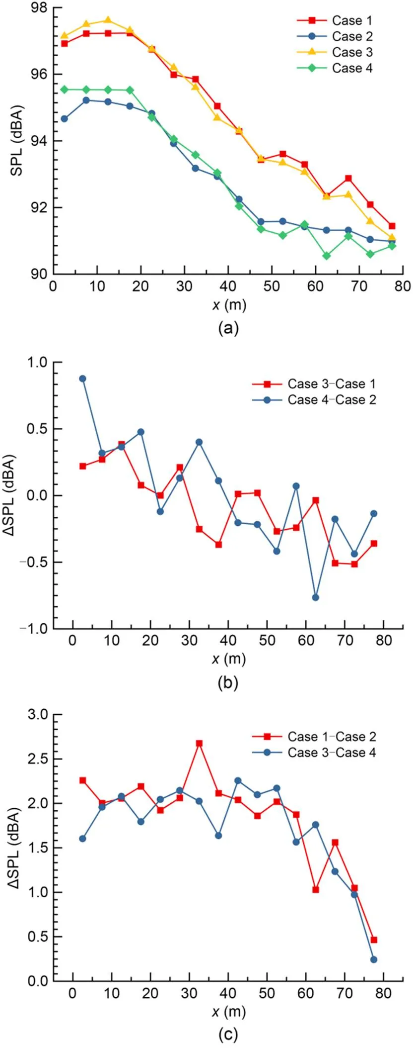
Fig. 13 Aerodynamic noise sound pressure level radiated by the vehicle to each measuring point: (a) results of the four GSSs; (b) difference between whether the wheel pair rotated or not; (c) difference between whether the ground was moving or not. SPL represents the A-weighted sound pressure level (dBA) and the reference quantity is 2×10-5 Pa

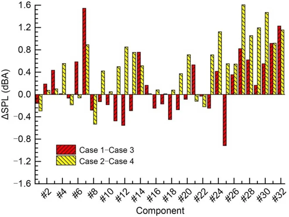
Fig. 14 Histogram of the difference in between the "rotating wheel" and "stationary wheel"

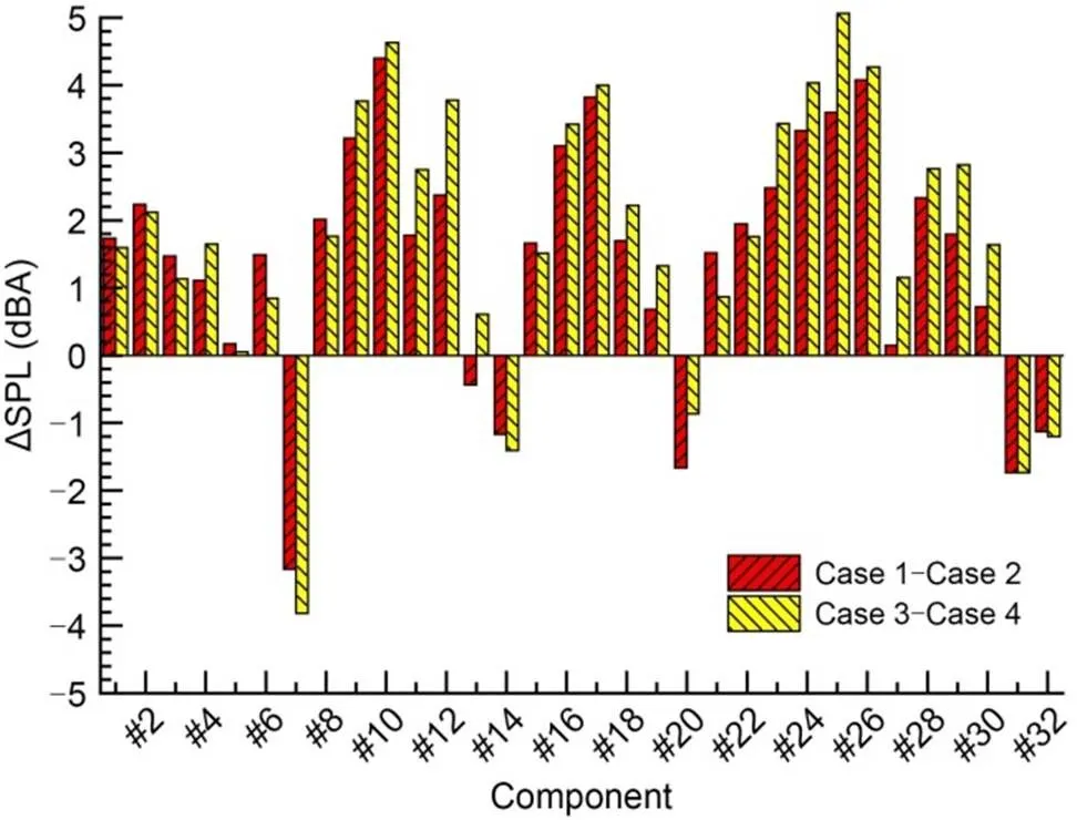
Fig. 15 Histogram of the difference in between the "moving ground" and "stationary ground"

5.2 Frequency characteristics

In this section, we discuss the influence of the four GSSs on the characteristics of the aerodynamic noise radiated by the whole car and its components. We discuss the influence of the aerodynamic noise spectrum characteristics in detail for the whole car, the bottom of the head/tail car streamlined.

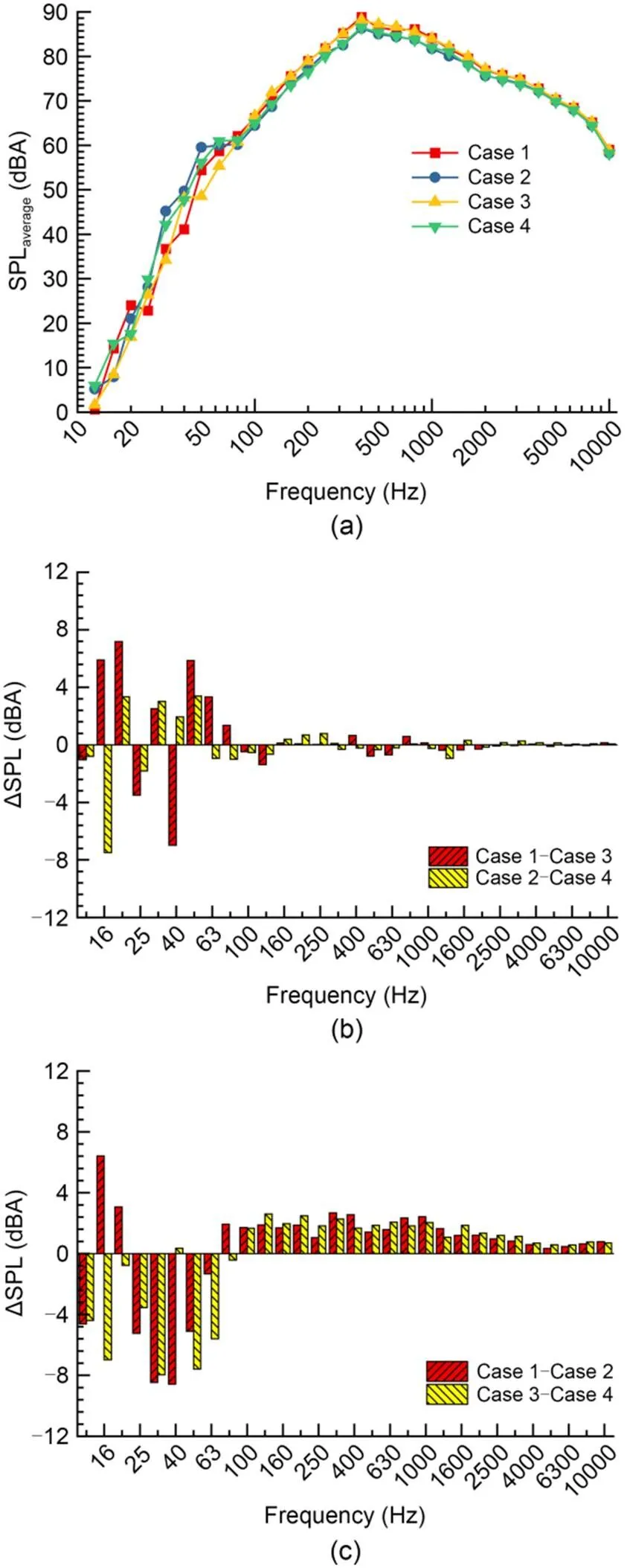
Fig. 16 spectrum curve radiated by the whole car: (a) result of the four GSSs; (b) value of the difference between "rotating wheel" and "stationary wheel"; (c) value of the difference between "moving ground" and "stationary ground"

According to Figs. 17 and 18, the spectrum curves of the above-mentioned components calculated by the four GSSs were identical, showing the distribution laws as small at both ends and large in the middle. However, the radiation of the components calculated by the four GSSs in each frequency band was quite different.

Fig. 17 spectral curve radiated by the bottom of the head car streamlined: (a) result of the four GSSs; (b) value of the difference between "rotating wheel" and "stationary wheel"; (c) value of the difference between "moving ground" and "stationary ground"

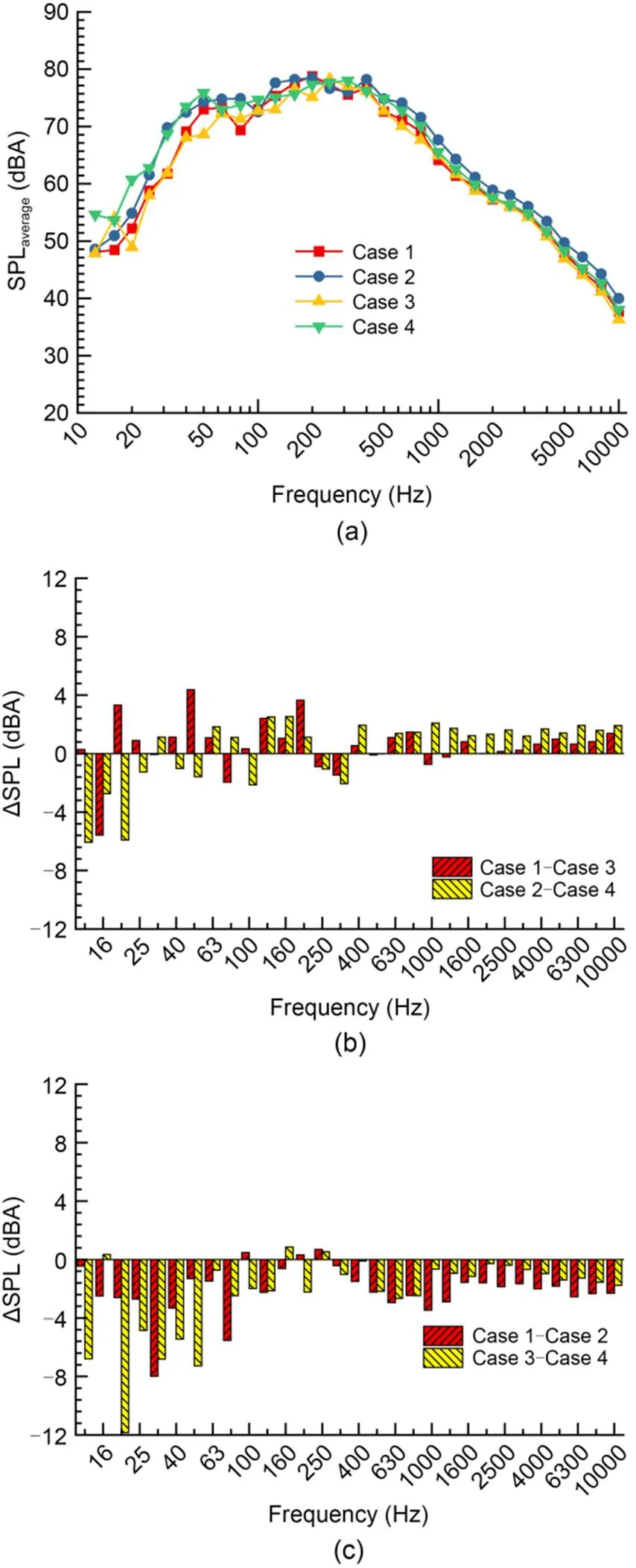
Fig. 18 spectral curve radiated by the bottom of the tail car streamlined: (a) result of the four GSSs; (b) value of the difference between "rotating wheel" and "stationary wheel"; (c) value of the difference between "moving ground" and "stationary ground"

The "moving ground" condition increased the velocity amplitude of the flow beneath the train, the scale of the vortex, the number of vortex groups transported downstream, and the tendency of the vortex group beneath the train to move to both sides of the train. This phenomenon did not appear in the "moving ground" condition, which is why the aerodynamic noise sources of the high-speed train and the noise intensity and frequency characteristics of the far field radiation were visibly different in the "stationary ground" and "moving ground" conditions.

6 Conclusions

In this study, we investigated the influence of four GSSs on the flow structure of a high-speed train, the sources of noise, and the far field radiation noise. Whether the wheel rotated or not and whether the ground moved or not hardly affected the flow field above the roof of the train. They affected mainly the flow field at the bottom of the train, where they had little effect on the aero-acoustic performance of the upper parts of the train, but had a significant effect on the aero-acoustic performance of the lower parts of the train. The effect of the wheels on the equivalent sound power of the whole train was less than 5%, but the effect of the ground movement condition on the equivalent sound power of the train was more than 15%. The average level of influence of rotation or non-rotation of the wheelset on the sound pressure level of aerodynamic noise was 0.3 dBA, while the level of influence of ground movement or not was 1.8 dBA. Wheelset rotation and ground movement mainly affected the equivalent sound power of the sound source and the sound pressure level below 100 Hz.

Considering that "wheelset rotation" increased the instability of numerical calculation, we suggest that only "ground slip" should be considered in the numerical calculation of the aerodynamic noise of high-speed trains. Considering that the ground was stationary in the acoustic wind tunnel experiment, we suggest that the experimental results of the high-speed train should be corrected appropriately in an acoustic wind tunnel.

This work is supported by the National Natural Science Foundation of China (No. 52272363) and the Foundation of the Key Laboratory of Aerodynamic Noise Control (No. ANCL20200302), China.

Xiaoming TAN designed the research. Xiaohong ZHANG and Zhigang YANG processed the corresponding data. Xiaoming TAN wrote the first draft of the manuscript. Linli GONG helped to organize the manuscript. Linli GONG revised and edited the final version.

Xiaoming TAN, Linli GONG, Xiaohong ZHANG, and Zhigang YANG declare that they have no conflict of interest.

Kouroussis G, Zhu SY, Vogiatzis K, 2021. Noise and vibration from transportation., 22(1):1-5. https://doi.org/10.1631/jzus.A20NVT01

Kwon HB, Park YW, Lee DH, et al., 2001. Wind tunnel experiments on Korean high-speed trains using various ground simulation techniques., 89(13):1179-1195. https://doi.org/10.1016/S0167-6105(01)00107-6

Liang XF, Liu HF, Dong TY, et al., 2020. Aerodynamic noise characteristics of high-speed train foremost bogie section., 27(6):1802-1813. https://doi.org/10.1007/s11771-020-4409-8

Liu JL, Zhang JY, Zhang WH, 2013. Study of computational method of far-field aerodynamic noise of a high-speed train considering ground effect., 30(1):94-100 (in Chinese). https://doi.org/10.7511/jslx201301016

Liu W, Guo D, Zhang Z, et al., 2019. Effects of bogies on the wake flow of a high-speed train., 9(4):759. https://doi.org/10.3390/app9040759

Paz C, Suárez E, Gil C, 2017. Numerical methodology for evaluating the effect of sleepers in the underbody flow of a high-speed train., 167:140-147. https://doi.org/10.1016/j.jweia.2017.04.017

Wang SB, Burton D, Herbst A, et al., 2018. The effect of bogies on high-speed train slipstream and wake., 83:471-489. https://doi.org/10.1016/j.jfluidstructs.2018.03.013

Tan XM, Liu HF, Yang ZG, et al., 2018. Characteristics and mechanism analysis of aerodynamic noise sources for high-speed train in tunnel., 2018:5858415. https://doi.org/10.1155/2018/5858415

Tyll JS, Liu D, Schetz JA, et al., 1996. Experimental studies of magnetic levitation train aerodynamics., 34(12):2465-2470. https://doi.org/10.2514/3.13425

Xia C, Shan XZ, Yang ZG, 2016. Influence of ground configurations in wind tunnels on the slipstream of a high-speed train. The 8th International Colloquium on Bluff Body Aerodynamics and Applications.

Xia C, Shan XZ, Yang ZG, 2017. Comparison of different ground simulation systems on the flow around a high-speed train., 231(2):135-147. https://doi.org/10.1177/0954409715626191

Yi SH, Zou JJ, Wu GF, et al., 1997. Experimental investigation for ground effects of the high speed train models on a plate with uniform boundary layer suction., 11(2):95-100 (in Chinese).

Zhang J, Li JJ, Tian HQ, et al., 2016. Impact of ground and wheel boundary conditions on numerical simulation of the high-speed train aerodynamic performance., 61:249-261. https://doi.org/10.1016/j.jfluidstructs.2015.10.006

Zhu JY, Hu ZW, Thompson DJ, 2017. The effect of a moving ground on the flow and aerodynamic noise behaviour of a simplified high-speed train bogie., 5(2):110-125. https://doi.org/10.1080/23248378.2016.1212677

Electronic supplementary materials

Sections S1–S3, Figs. S1–S5, and Eqs. (S1)–(S3)

地面效应对高速列车流场结构及气动噪声的影响

谭晓明1,2，龚林立1，张晓红1，杨志刚2

1湖南理工学院，机械工业激光磨削复合智能制造与服役性能优化重点实验室，中国岳阳，414000；2中南大学，轨道交通安全教育部重点实验室，中国长沙，410075

高速列车作为高速地面交通工具，不可避免地会遇到地面效应问题。地面效应模拟一直是高速列车风洞试验的技术难点。地面效应现象的准确模拟对高速列车空气动力学和气动噪声的预测精度有很大的影响。通过对比4种地面模拟系统（GSS）的流声场结果，研究不同GSS对流场结构、气动声源和远场辐射噪声特性的影响规律，为高速列车声学风洞试验提供指导。

1. 搭建高速列车地面模拟系统，模拟不同边界条件；2. 明确轮对旋转与地面滑移对高速列车气动噪声幅值的相对增量及影响频率范围。

1. 在仿真系统中建立“移动地面+旋转轮对”、“静止地面+旋转轮对”、“移动地面+静止轮对”和“静止地面+静止轮对”四种地面模拟系统；2. 采用大涡模拟和旋度声学积分方程，对高速列车的流声场结果进行模拟；3. 通过对比4种GSS的流声场结果，研究不同GSS对流场结构、气动声源和远场辐射噪声特性的影响规律。

1. 移动地面和旋转轮对是影响列车底部气动声学性能的主要因素；2. 旋转轮对对整车等效声源功率的影响不大于5%，且移动地面对整车等效声源功率的影响大于15%；3. 旋转轮对对整车辐射声压级的平均影响为0.3 dBA，且运动地面对整车辐射声压级的平均影响为1.8 dBA；它们主要影响100 Hz以下的气动声学性能。

高速列车；气动声学；流场结构；大涡模拟；移动地面；旋转轮对

https://doi.org/10.1631/jzus.A2300034

https://doi.org/10.1631/jzus.A2300034

Zhigang YANG, yangzg1976@163.com

Zhigang YANG, https://orcid.org/0000-0001-7255-7324

Received Jan. 16, 2023;

Revision accepted May 27, 2023;

Crosschecked Jan. 5, 2024

© Zhejiang University Press 2024