Dendroclimatological study of Sabina saltuaria and Abies faxoniana in the mixed forests of the Qionglai Mountains,eastern Tibetan Plateau

Teng Li · Jianfeng Peng · Tsun Fung Au ·Jingru Li · Jinbao Li · Yue Zhang

Abstract Tree-ring chronologies were developed for Sabina saltuaria and Abies faxoniana in mixed forests in the Qionglai Mountains of the eastern Tibetan Plateau.Climategrowth relationship analysis indicated that the two co-existing species reponded similarly to climate factors,although S.saltuaria was more sensitive than A. faxoniana.The strongest correlation was between S. saltuaria chronology and regional mean temperatures from June to November.Based on this relationship,a regional mean temperature from June to November for the period 1605–2016 was constructed.Reconstruction explained 37.3% of the temperature variance during th period 1961–2016.Six major warm periods and five major cold periods were identified.Spectral analysis detected significant interannual and multi-decadal cycles.Reconstruction also revealed the influence of the Atlantic Multi-decadal Oscillation,confirming its importance on climate change on the eastern Tibetan Plateau.

Keywords Tree-ring analysis · Mixed forests ·Dendroclimatology · Qionglai Mountains

Introduction

The Tibetan Plateau has long been considered as the roof of the world,and is the largest plateau in China and the world’s highest.The Plateau affects climate at regional and global scales and receives considerable attention in the study of large-scale climate change (Liu and Zhang 1998;Liu and Chen 2000;Liu et al.2009;Yang 2012).The Plateau is one of the more sensitive and vulnerable regions in terms of climate change (IPCC 2013;Zhu et al.2016;Li and Li 2017).However,scarce instrumental records make it difficult to fully understand the effects of climate change on the Plateau.Proxy records are essential to studies of long-term climate change on the Plateau.Among them,tree-rings have been widely used owing to the annual resolution,accurate dating,and high sensitivity to climate in many regions around the globe (Fritts 1976;Schweingruber 1996;Shao 1997;Gou et al.2010;Peng et al.2014).Numerous dendroclimatological studies have been carried out on the Tibetan Plateau focused on temperature (Bräuning and Mantwill 2004;Gou et al.2007;Fan et al.2010;Duan and Zhang 2014;He et al.2014;Wang et al.2014;Liang et al.2016;Li and Li 2017;Li et al.2018,2020,2021) and precipitation (Sheppard et al.2004;Shao et al.2005;Liu et al.2006b;Yang et al.2014).

The eastern areas of the Tibetan Plateau,with average altitudes above 3000 m a.s.l.,is the transition zone from the Plateau to the Sichuan Basin.To some extent,abundant sunshine makes up for the heat loss at high altitudes so that trees grow to a higher elevations,an optimal condition for maximizing climate signals in tree-rings.Therefore,the eastern plateau area is an ideal location for tree-ring studies of long-term climate change (Li et al.2010).In past decades,climate reconstructions have been carried out in the eastern Tibetan Plateau,especially using average temperatures(Wu et al.2005;Duan et al.2010;Li et al.2010,2014;Yu et al.2012b;Xiao et al.2013a,2015a,b;Deng et al.2014),maximum temperatures (Qin et al.2008;Xiao et al.2013b;Zhu et al.2016) and minimum temperatures (Shao and Fan 1999;Song et al.2007;Yu et al.2012a).These studies haven shown that tree growth in the eastern Tibetan Plateau is largely limited by temperature.Nevertheless,these studies have only revealed past climate changes in parts of the plateau and were largely based on tree species such asPicea asperataMast.,Abies georgei,orAbies fabri(Mast.)Craib.Other tree species in the mixed forests can be further used for dendrochologoical studies in the region.

The aims of this study were to: (1) develop tree-ring width chronologies of the Sichuan juniper (Sabina saltuariaRehd.&Wilson) and Farges’ fir (Abies faxonianaRehd.&Wilson) on the eastern Tibetan Plateau,and compare their responses to climate factors;(2) reconstruct past climate changes based on climate-tree growth relationships;and (3)identify possible driving mechanisms of climate change in the region.

Materials and methods

Study site

The study site is located in the Liangtai valley (31.39° N,102.89° E,at 3555 m a.s.l.) in the central Qionglai Mountains on the eastern Plateau (Fig.1).This region has cool summers and cold winters,with annual mean temperatures of 6.9–11 °C and annual total precipitation of 650–1000 mm.There are extensive mixed forests in the valley,and the dominant vegetation includesSibiraea laevigata,Rhododendron simsii,Larix mastersiana,Salix cupularisandLonicera japonicaThunb.,similar to nearby Bipeng valley (Lin et al 2019).Dark brown soil occurs on slope deposits (Wu et al.2010).

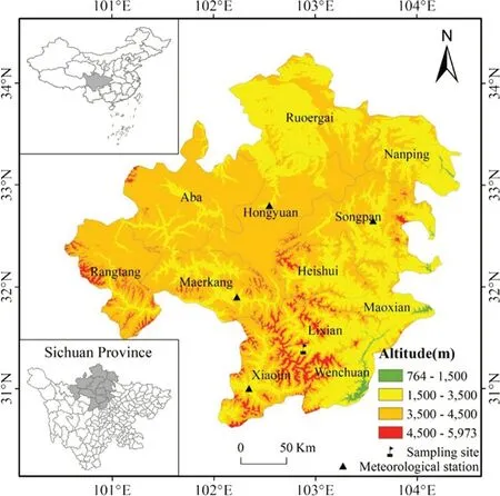
Fig.1 Location of the study site (flag) and nearby meteorological stations (triangles)

Tree-ring data

Tree core samples fromS.saltuariaandA.faxonianawere collected in June 2017.One or two cores were taken from canopy-dominant,healthy trees in different directions at breast height (1.3 m above ground) using 5.15 mm increment borers.Twenty-two and 37 cores from 11 and 19 trees were obtained fromS.saltuariaandA.faxoniana,respectively.

Standard dendrochronological methods of Cook and Kairiukstis (1990) were followed to prepare the core samples.The samples were air-dried,mounted on wooden slots,sanded with different grades of sandpaper (150–800 meshs)until cells and individual tracheids within annual rings were clearly discernible under the microscope.After visually cross-dating,ring widths were measured using the Velmex measuring system with a precision of 0.001 m (Bloomfield,NY,USA).The quality of cross-dating and measurement accuracy were statistically checked by the COFECHA program (Holmes 1983).Cores with low inter-series correlation were removed to prevent adding noise in chronology development.Finally,19 and 34 cores from 10 and 19 trees were retained fromS.saltuariaandA.faxoniana,respectively(Table 1).

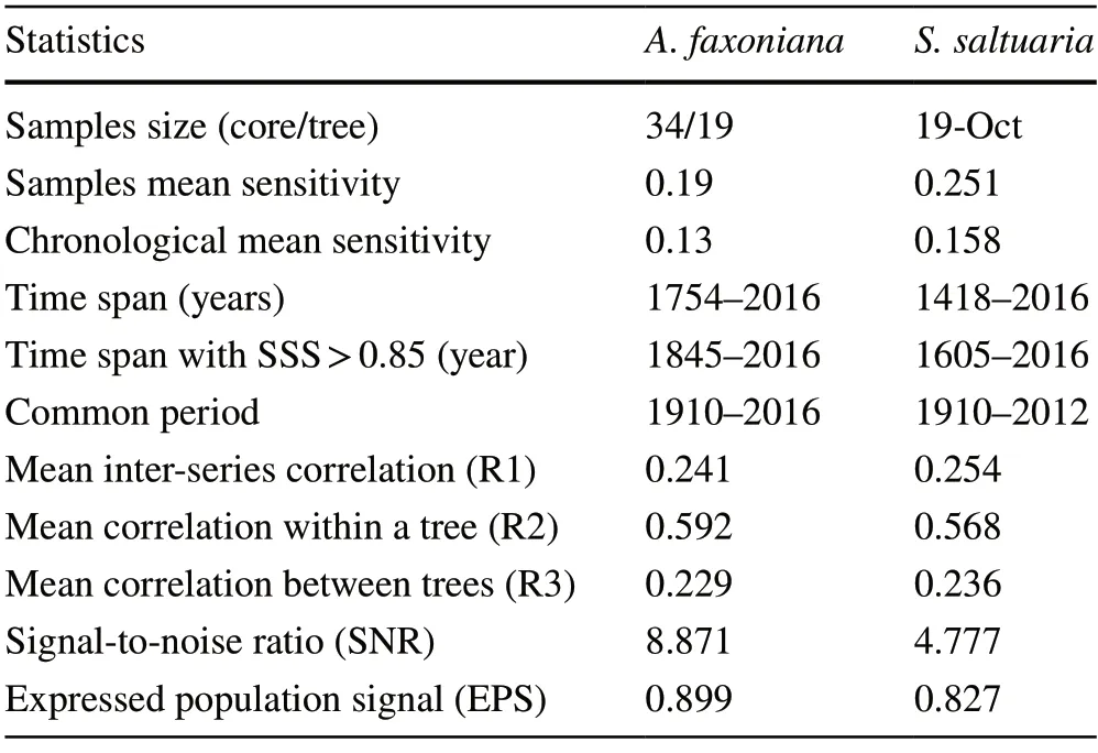
Table 1 Statistical characteristics of tree-ring chronologies of the two species

Individual ring-width series were detrended to reduce the loss of low-frequency signals from tree age and stand dynamics by fitting a conservative negative exponential curve or linear curve with negative or zero slope using the ARSTAN program (Cook and Holmes 1986).The robust biweight mean was used to build the chronology from the standardized tree-ring series (Cook and Kairiukstis 1990).The subsample signal strength (SSS) of 0.85 was employed to identify the reliable period of the chronologies (Wigley et al.1984).The statistical characteristics of the tree-ring width standard chronologies are shown in Table 1 and the chronologies in Fig.2.

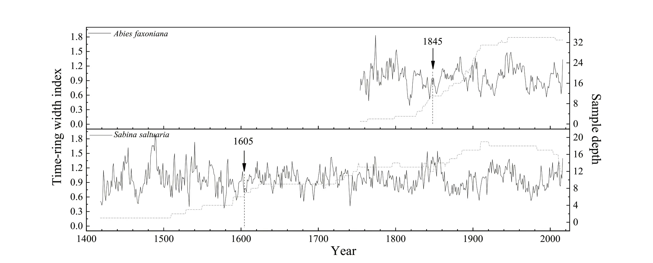
Fig.2 Tree-ring width chronology (solid line) and sample depth (dotted line) from A. faxoniana and S. saltuaria.Vertical dashed line denotes SSS >0.85

Climate data

Climate data were obtained from four meteorological stations (Xiaojin,Maerkang,Hongyuan and Songpan,Table 2)from the China Meteorological Data Sharing Service System(https:// data.cma.cn/).Monthly mean (Tmean),maximum(Tmax) and minimum (Tmin) temperatures and monthly total precipitation (P) were used.To minimize spatial heterogeneity,records from the four meteorological stations were averaged to build regional monthly temperature and precipitation records.Based on climate data from 1961 to 2016,the regional annual Tmean was approximately 7.2 °C,with the monthly Tmean above 0 °C from February to November.Annual total precipitation was approximately 720 mm largely concentrated in May to September (Fig.3).

Table 2 Information of four weather stations near the sampling site

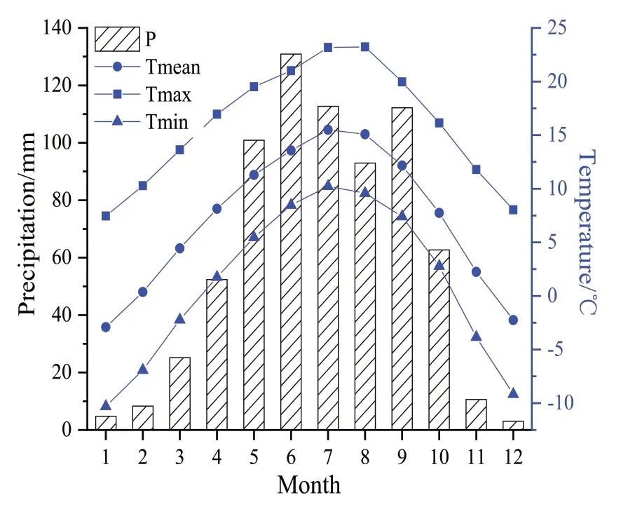
Fig.3 Monthly mean (Tmean),maximum (Tmax),minimum (Tmin)temperatures and monthly total precipitation (P) from regional meteorological data (1961–2016).Months of 1–12 indicate January to December

Statistical analysis

The relationship of the two chronologies of the two species with regional climatic factors were analyzed using Dendro-Clim2002 (Biondi and Waikul 2004),with 21 months of window from the previous March to the current November.Based on the climate-growth relationship,a simple linear regression model (Cook and Kairiukstis 1990) was developed for reconstruction.

The traditional split sample calibration-verification method tested the reliability of the reconstruction model(Cook and Kairiukstis 1990).Statistical parameters,including Pearson’s correlation coefficient (r),the coefficient of determination (R2),the sign test (ST),the reduction of error(RE),the coefficient of efficiency (CE) and the Durbin–Watson (D/W) test,were used to evaluate the reconstruction model (Fritts 1976;Cook and Kairiukstis 1990).Positive values of RE and CE are considered to be good indicators of an appropriate model (Cook et al.1999).

An 11-year moving average method was applied to explore multidecadal changes of the reconstruction.Spectral analyses were performed using the Multi-Taper Method(MTM;Mann and Lees 1996) and wavelet analysis (Torrence and Compo 1998) to explore the periodic variations of the reconstructed series.Spatial correlations between the observed and reconstructed series and 0.5° × 0.5° gridded CRU TS4.03 temperature data (Harris et al.2014) were calculated using the KNMI climate explorer (http:// clime xp.knmi.nl/) to understand regional representativeness.In order to investigate the impacts of global sea surface temperatures on climate varaiblity in the study area,the global extended reconstructed sea surface temperature version 4 dataset (ERSST v4) was adopted for spatial correlations(Huang et al.2015).

Results

Climate-growth relationships of the two species

Growth ofA.faxonianaandS.saltuariawas positively correlated with most regional temperature parameters.There were significant positive correlations between annual rings ofA.faxonianaand regional Tmean in the previous April and October and the current October (Fig.4a).The growth ofA.faxonianawas also positive with regional Tmax in the previous September and October and the current October(Fig.4b).Significant positive correlations were found with regional Tmin in the previous April and October and the current October (Fig.4c).

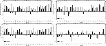
Fig.4 Correlations between climate factors (Tmean,Tmax,Tmin,P)and chronologies of A. faxoniana (Af) and S. saltuaria (Ss) during 1961–2016.Months of p3–p12 indicate previous March to previous December;Months of C1–C11 indicate current January to current November;C6–11 (current June to November) represents the target season for reconstruction;horizoental dashed lines denote 95% confidence level

Growth ofS.saltuariahad similar relationships with temperatures;it was significantly positive with regional Tmean in the previous March,June,and November,and the current February,June–August,and October–November (Fig.4a).Growth was positively related to the regional Tmax in the previous June and December,and the current February,June–July,and October–November (Fig.4b) as well as regional Tmin in the previous March–April,June,and the current February,April,July–August,and October–November (Fig.4c).At the same time,growth of both species was weakly related with precipitation despite negative correlations withS.saltuariain the previous September and withA.faxonianain the current June (Fig.4d).

Generally seasonal climate was more likely to influence growth than monthly climatic variables.Therefore,correlations between different combinations of regional monthly climatic factors and chronologies ofA.faxonianaandS.saltuariawere further explored to determine if there was a limiting climatic factor on growth.The results show that the chronology ofS.saltuariahad the highest correlation with regional Tmean in the current June-November period (T6-11,r=0.610,p<0.001),indicating that it was the main limiting factor onS.saltuariagrowth.

Regional T6-11 reconstruction

With the limiting factor of regional T6–11onS.saltuariagrowth,a simple linear regression model between theS.saltuariachronology and regional T6-11was developed to reconstruct past temperature changes.The model is:

where T6-11is the regional mean temperature from June to November,Wtis the ring-width index at year t.The reconstruction model accounted for 37.3% (36.1% after adjusting for the degree of freedom) of the regional Tmean variance from 1961 to 2016.The D/W test value (Durbin and Watson 1950) was 1.647 (Table 3),which indicated that there was no significant autocorrelation or linear trend in the residuals.The split-sample calibration and verification method tested the stability and reliability of the reconstruction model (Table 3).The generally positive RE and CE values for verification indicated that the regression model was reliable for reconstruction (Cook et al.1999),although the CE value was slightly negative during 1961–1988.Almost all of these statistical parameters showed that the reconstruction model was stable and reliable.There was good consistency between the reconstructed and the observed series during 1961–2016 (Fig.5a).Therefore,regional T6–11since 1605 AD was reconstructed for the study region using the above regression model (Fig.5b).

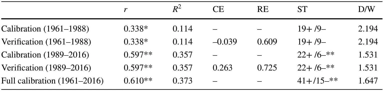
Table 3 Calibration and verification statistics for regional T6–11 reconstruction

Fig.5 a Comparison of observed (solid line) and reconstructed (dashed line) regional T6-11 during 1961–2016;b the reconstructed (thin line)regional T6–11 and its 11-year moving average (thick line) during 1605–2016

Regional temperature variations over the past 412 years

Based on the above regression model,regional T6-11from 1605 to 2016 was reconstructed.Temperatures ranged from 10.3–12.1 °C with its mean of 11.1 °C (Fig.5b).Based on mean ± σ,the extremely high temperature was defined as exceeding 11.5 °C and extremely low temperature below 10.8 °C.Therefore,the extremely high and low temperature years accounted for 15% (63 years) and 17% (71 years) of the past 412 years,respectively.The top five warmest years were 1854,1841,1773,1848,and 1717,and the five coldest years were 1741,1681,1975,1908 and 1694,respectively.Based on the 11-year moving average of the reconstructed series,there were six major warm periods (1612–1673,1702–1737,1754–1780,1832–1863,1916–1959,2000–2016) and five major cold periods (1674–1701,1738–1753,1781–1831,1864–1915,1960–1999) in the past 412 years.

Periodic variation of the reconstructed series

Multi-Taper Method (MTM) spectral analysis indicated several important periodicities in the reconstructed temperature series (Fig.6).Significant periodic oscillations of interannual (2.0–2.2a,3.6a,7.0a,9.5a) and multi-decadal(75.6–95.1a) timescales at 95% significance were found over 1605–2016.Wavelet analysis showed that the interannual cycles were the main periods of temperature change over the full reconstruction period,while the multi-decadal cycle was most pronounced over 1800–2000 (Fig.7).

Fig.6 MTM spectral analysis of the reconstructed T6–11 1605–2016.Solid and dashed lines denotes 90% and 95% confidence levels respectively

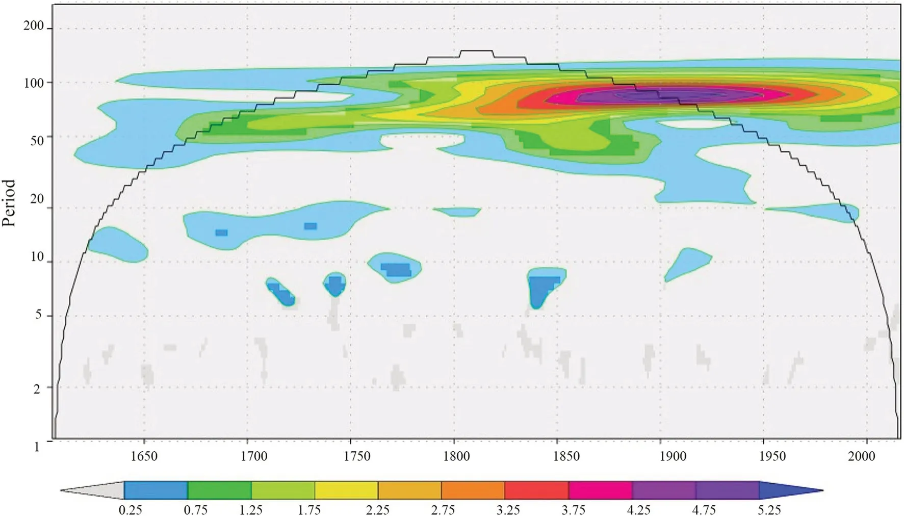
Fig.7 Wavelet analysis of the reconstructed T6–11 during 1605–2016

Discussion

Climate-growth response of the two species

Based on correlations between tree-ring chronologies and regional climatic factors,that temperature in most months was positively correlated withS.saltuariaandA.faxonianagrowth (Fig.4).The study area is influenced by the monsoon climate with high rainfalls and cool summers due to the terrain.Rainy weather with increased cloud cover reduces solar radiation and also lowers temperatures.Therefore,temperatures in the growing season,especially during June–November,had considerable influence on regional tree growth (Yu et al.2012b;Zhu et al.2016).Increasing temperatures in the growing season enhances photosynthesis and stimulates cell division,is conducive to radial growth when a minimum temperature threshold is reached (Shao and Fan 1999;Qin et al.2008;Xiao et al.2015a;Li et al.2017).Therefore,temperature was the critical factor controlling tree growth in the eastern Tibetan Plateau when precipitation was abundant in the growing season.

Spatial representativeness of the reconstruction

To explore the regional representativeness of the reconstructed T6–11,a spatial correlation analysis was performed using the actual and reconstructed T6–11with 0.5° × 0.5°gridded CRU TS4.03 temperature from 1961 to 2016(Fig.8).The results indicate that spatial correlation patterns are consistent between the actual and reconstructed T6–11series over the eastern Tibetan Plateau,albeit the correlations are slightly weaker for the reconstruction.Both series have significant positive correlations,suggesting that the reconstructed T6–11can represent regional temperature changes over the past four centuries.

Fig.8 Spatial correlations of the a actual and b reconstructed T6–11 with CRU TS4.03 temperatures during 1961–2016.The star denotes the sampling site

To validate regional representativeness of the reconstructed T6–11,annual temperatures from the previous September to the current August (T9–8) in Songpan (Li et al.2014) and the July temperature (T7) reconstruction in Maerkang (Yu et al.2012b) were compared (Fig.9a,b,c).Three reconstructions exhibit similar temperature variations: the warm periods of 1700s–1730s,1840s–1850s,1940s–1960s,2000s–2010s,and the cold periods of 1670s–1690s,1810s–1830s,1970s–1990s.Similar results have also been noted in other regions of the eastern Tibetan Plateau (Shao and Fan 1999;Yu et al.2012a;Xiao et al.2013a,2015a).

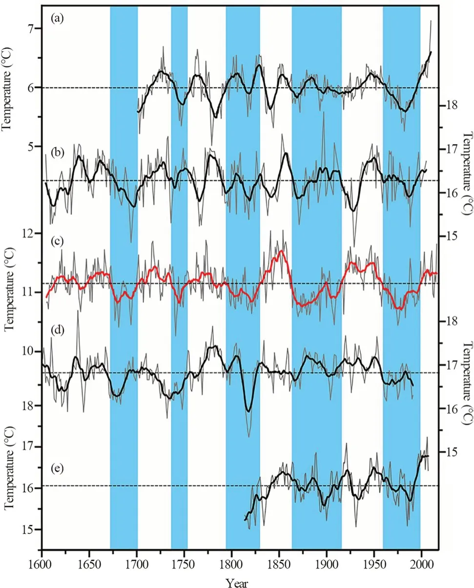
Fig.9 Comparison of a T9–8 in Songpan (Li et al.2014),b T7 in Mearkang (Yu et al.012b),c T6–11 in Liangtai valley (this study),d T2-6 in Kathmandu (Cook et al.2003),e T5–9 in Arxan,Inner Mongolia (Liu et al.2012).Bold lines denote 11-year moving average in each panel,blue shading denotes major cold periods in the T6-11 reconstruction

To verify the spatial representativeness of the reconstructed T6–11at a larger scale,it was further compared with the February–June (T2–6) reconstruction in the Himalayas (Cook et al.2003),and the May–September (T5–9)reconstruction in Arxan,Inner Mongolia (Liu et al.2012).The three reconstruction series were consistent of the low temperature periods in the 1810s–1830s and 1970s–1990s,and in the warm period in the 1940s–1960s,suggesting a synchronized temperature change at a large scale (Fig.9c,d,e).

The tree-ring based temperature reconstructions are also consistent with the advance and retreat of the Hailuogou Glacier (Li et al.2008,2009;Liu et al.2006a;Xiao et al.2015a) on the eastern Tibetan Plateau.The glacier retreated during the 1930s–1960s,corresponding to a warm period in the T6-11reconstruction.During the 1970s–1980s,the glacier was relatively stable or retreated slowly,reflecting a continuous period of low temperatures.Since the mid-1980s,the glacier has been in a stage of rapid retreat and the reconstructed T6–11showed temperature increases due to global warming (IPCC 2013).

Possible driving mechanisms

The results of MTM and wavelet analyses revealed significant cycles in the reconstructed temperatures (Figs.6,7).The 2–7a and 9.5a periods were consistent with the periodic changes of the El Nino–Southern Oscillation (Song et al.2007;Li et al.2010;Yu et al.2012b;Xiao et al.2013b;Zhu et al.2016) and solar activity (Xiao et al.2013b,2015b).The 75.6–95.1a cycle may be related to the Atlantic Multidecadal Oscillation (Zhu et al.2016).

Oceans regulate atmospheric circulation and world climate variability (Cai and Liu 2017),and are strongly connected with regional climates.Spatial correlations of the observed and reconstructed T6–11with global sea surface temperature during 1961–2016 showed a similar spatial correlation,with positive correlations in the western Pacific and North Atlantic oceans (Fig.10).The relationship of our temperature reconstructions were further vertified with the Atlantic Multidecadal Oscillation by calculating their correlations over the period 1880–2016.The results indicate that our temperature reconstructions had a positive correlation (r=0.385,p<0.01) during the period.This is consistent with studies showing the influence of the Atlantic Multidecadal Oscillation on the eastern Tibetan Plateau (Wang et al.2014;Liang et al.2016;Li and Li 2017;Li et al.2021).The warm-phase of the Atlantic Multidecadel Oscillation in summer can trigger positive geopotential height anomalies in the subtropical western Pacific and strong subtropical anticyclones,which further strengthen the East Asian summer monsoon (Lu et al.2006;Wang et al.2009).In addition,the warm-phase in winter can cause strong midlatitude westerly winds and extend the North Atlantic low surface air pressure to the Eurasian continent,leading to a weakened East Asian winter monsoon (Dong et al.2006;Li and Bates 2007;Wang et al.2009;Ding et al.2014).The warm-phase may also heat the Asian continent troposphere via the mid-and highlatitudes Rossby wave propagation (He et al.2014;Wang et al.2014).Therefore,it may have a crucial influence on temperature variability in the region.

Fig.10 Spatial correlations of the a observed and b reconstructed T6–11 with global ERSST v4 SSTs in T6–11 over the period 1961–2016

Conclusions

In this study,tree-ring width chronologies ofS.saltuariaandA.faxonianafrom the mixed forests on the eastern Tibetan Plateau were developed.The results indicate that the radial growth of both species was strongly influenced by temperature.The strongest relationship was found between annual rings ofS.squamataand regional mean temperatures from June to November (T6–11).Based on this relationship,a regional T6-11was reconstructed for the period 1605–2016.Spatial correlation analysis and comparison with other temperature reconstructions revealed that our reconstruction represented large-scale temperature changes on the plateau and showed a strong warming trend since the 1980s,suggesting that tree growth tracks well the warming signals in the region.Moreover,our records exihibit a linkage with the Atlantic Multidecadel Oscillation,providing new evidence on its influence on climate change over the eastern Tibetan Plateau.

Open AccessThis article is licensed under a Creative Commons Attribution 4.0 International License,which permits use,sharing,adaptation,distribution and reproduction in any medium or format,as long as you give appropriate credit to the original author(s) and the source,provide a link to the Creative Commons licence,and indicate if changes were made.The images or other third party material in this article are included in the article’s Creative Commons licence,unless indicated otherwise in a credit line to the material.If material is not included in the article’s Creative Commons licence and your intended use is not permitted by statutory regulation or exceeds the permitted use,you will need to obtain permission directly from the copyright holder.To view a copy of this licence,visit http://creativecommons.org/licenses/by/4.0/.