Knowledge Transfer Learning via Dual Density Sampling for Resource-Limited Domain Adaptation
2023-12-22ZefengZhengLuyaoTengWeiZhangNaiqiWuandShaohuaTeng
Zefeng Zheng, Luyao Teng, Wei Zhang, Naiqi Wu,,, and Shaohua Teng,,
Abstract—Most existing domain adaptation (DA) methods aim to explore favorable performance under complicated environments by sampling.However, there are three unsolved problems that limit their efficiencies: i) they adopt global sampling but neglect to exploit global and local sampling simultaneously; ii)they either transfer knowledge from a global perspective or a local perspective, while overlooking transmission of confident knowledge from both perspectives; and iii) they apply repeated sampling during iteration, which takes a lot of time.To address these problems, knowledge transfer learning via dual density sampling (KTL-DDS) is proposed in this study, which consists of three parts: i) Dual density sampling (DDS) that jointly leverages two sampling methods associated with different views, i.e., global density sampling that extracts representative samples with the most common features and local density sampling that selects representative samples with critical boundary information; ii)Consistent maximum mean discrepancy (CMMD) that reduces intra- and cross-domain risks and guarantees high consistency of knowledge by shortening the distances of every two subsets among the four subsets collected by DDS; and iii) Knowledge dissemination (KD) that transmits confident and consistent knowledge from the representative target samples with global and local properties to the whole target domain by preserving the neighboring relationships of the target domain.Mathematical analyses show that DDS avoids repeated sampling during the iteration.With the above three actions, confident knowledge with both global and local properties is transferred, and the memory and running time are greatly reduced.In addition, a general framework named dual density sampling approximation (DDSA) is extended, which can be easily applied to other DA algorithms.Extensive experiments on five datasets in clean, label corruption(LC), feature missing (FM), and LC&FM environments demonstrate the encouraging performance of KTL-DDS.
I.INTRODUCTION
ARTIFICIAL intelligence (AI) applications are usually implemented based on a great deal of labeled samples that obey the same distributions.However, for an embedded device, it is very difficult to obtain the semantics of samples which we are interested in (called target samples).For example, an on-orbit satellite may collect a huge amount of data.Due to transmission delay and industrial cost, it is almost impossible to tag such real-time arrival data manually.
One promising way is to store sufficient labeled samples(called source samples) collected from crowdsourcing in a device.Then, the device can leverage such labeled source samples to train a classifier and tag the unlabeled target samples.This practice is known as domain adaptation (DA) and it attracts significant attention [1]–[5].The purpose of DA is to eliminate domain discrepancies between the source and target domains so that the classification knowledge of the source domain can be applied to the target domain [6]–[8].
In the past years, DA has made remarkable achievements in both shallow machine learning and deep learning fields [1],[9]–[16].In shallow machine learning, researchers usually apply some statistical learning methods that transform knowledge from the source to target domains.Practically, all the data in the source and target domains are trained at the same time.For example, Tianet al.explore local structural information and map the class centroids of two domains jointly [9].During the optimization process, a greedy strategy is applied to achieve unified learning of the knowledge.Wang and Breckon select a part of the “reliable” target samples, and train them progressively [17].Zhanget al.introduce guide subspace learning (GSL), which mines a low-rank reconstruction matrix for target samples through a two-stage learning strategy [11].As for deep learning methods, the data is usually divided into multiple batches and only a part of them (e.g.,one batch) is used to update the gradient value of the objective function in each iteration.Recently, Jianget al.propose resource efficient domain adaptation (REDA) for efficient learning [12].In REDA, the learned knowledge is transferred progressively from the features taken by a deep extractor to the ones by a shallow extractor.Consequently, the inference time for “easy samples” is reduced so that the computation time is reduced.Liet al.propose a dynamic domain adaptation (DDA) framework [13].In DDA, only a part of the highconfidence target samples are measured for training in each iteration.Hence, DDA reduces redundant calculations and achieves promising performance.Sharmaet al.propose a general approach called instance level affinity-based transfer(ILA) [15].ILA utilizes multi-sample contrastive (MVC) loss for instance-level transfer learning, which makes it easy to apply to other DA methods.
Although many heuristic algorithms are proposed to accelerate learning [12], [13], [17], [18],a general and efficient algorithm in shallow machine learning is still needed.For instance, when a virus mutates, we need to train a suitable model to detect such a virus in a short time.Although deep DA methods can achieve promising performance, we might prefer to develop a shallow DA method and detect the virus as quickly as possible (despite its limited recognition rate)1Generally, a deep learning method takes several hours or days, while a shallow learning method takes a few seconds or minutes..Hence, an efficient shallow algorithm is helpful in developing a rough detection mechanism for blocking the spread of viruses.
To improve the efficiency of an algorithm for DA, a typical practice is to employ global sampling or local sampling2Global sampling denotes that the samples are selected according to global metrics (e.g., the overall shape of the object, and the average distance to all the other samples), while local sampling denotes that by local metrics (e.g., a small area of the image, and the average distance to the other neighborhood samples).to extract a representative subset from a training set for training.Yet, existing algorithms commonly adopt some global sampling methods to select a part of the “reliable” samples for training [13], [17], [18].Despite their promising performance achieved, there are three unresolved issues that hinder the development of these effective methods:
1)Existing efforts[13],[17],[18]may adopt global sampling but neglect to exploit both global and local sampling simultaneously.In order to reduce the training scale, many algorithms develop some global sampling methods to estimate the whole distribution of the data.In [18], Zhaoet al.detect the target samples with high global densities and utilize them for training.Liet al.add the target samples with high predicted probability for training [13], [17].Since the global sampling methods extract the most common part of the distribution, these algorithms achieve a good performance.However, they neglect to detect the samples located at the classification boundaries, i.e., the samples with local properties.As a result, they may lead to under-fitting and fail in bridging the gap between domains.Hence, the performance is hindered.
2)Existing works[12],[13],[17]either learn the knowledge from a global perspective or a local perspective,while overlooking the transmission of the confident knowledge from both of them.Since the existing methods [12], [13], [17] adopt global sampling to extract representative samples, the knowledge with global properties is learned.In this case, one might utilize the manifold regularization on these sampled instances and learn local information from them [9].However, due to the ignorance of the samples with local properties, it is hard to extract classification knowledge with local characteristics as much as possible.As a result, performance might be deteriorated.
3)Existing works[12],[13],[17]inevitably apply repeatedsampling during iteration,which leads to a heavy time consumption.In SPL and DDA, a part of “reliable” target samples are selected for training.Although they achieve good performance, they need to calculate scores of the target samples in each iteration repeatedly.In large-scale training scenarios,the time for repeated sampling becomes the dominant computation burden in training.For instance, when training SPL on task Ar → Cl on Office-Home, about 6.69±0.12 seconds are required for sampling, and 0.97±0.02 seconds are required to learn the projection matrix in one iteration.When the number of iterations increases, sampling takes more and more time in the training process.In this case, avoiding repeated sample selection during iteration is an urgent problem, which can save a great deal of calculations.
To address the above three problems, we develop knowledge transfer learning via dual density sampling (KTL-DDS)in this study.KTL-DDS adopts both global and local sampling, avoiding repeated sample selection during iteration and learning the confident knowledge with global and local properties.
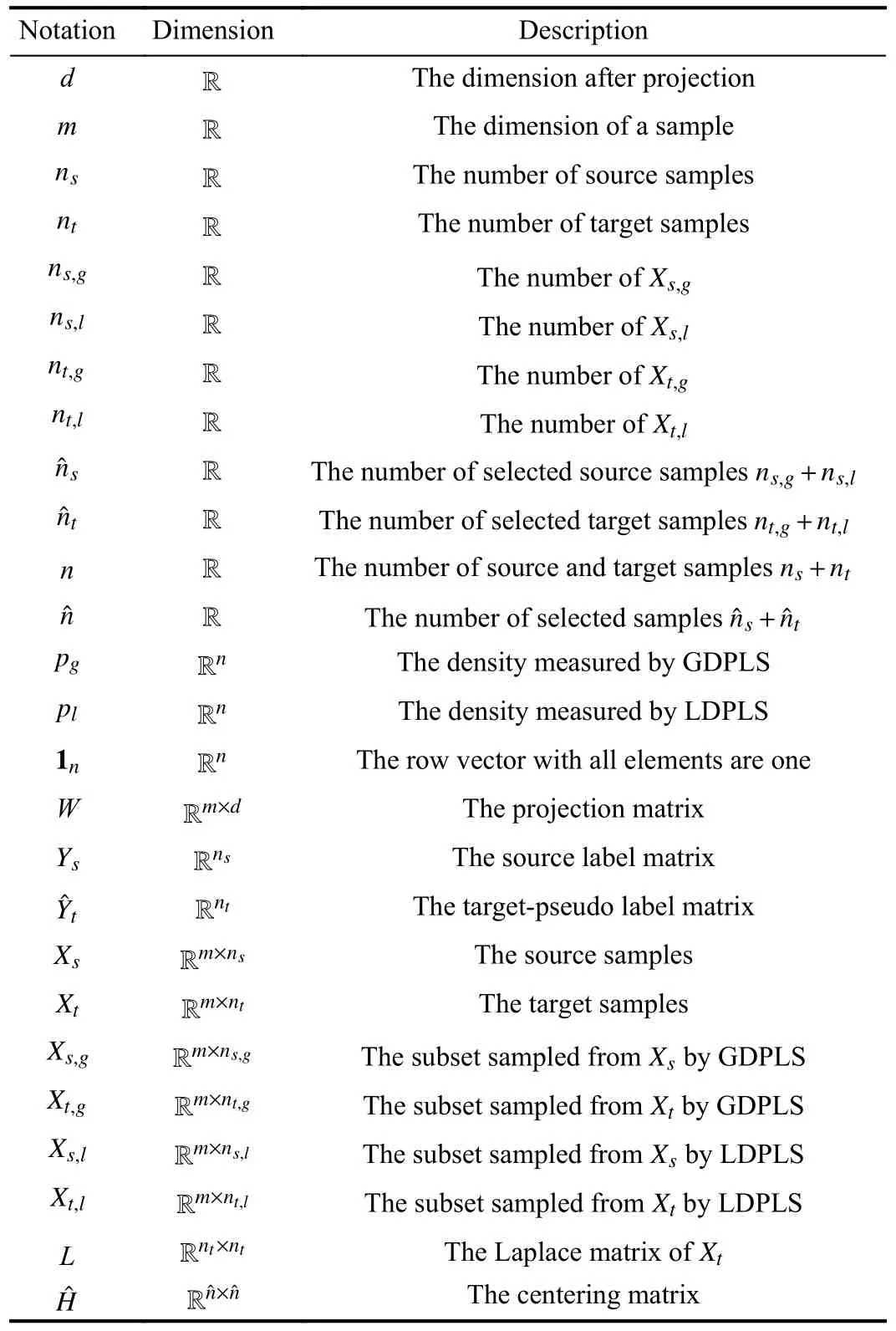
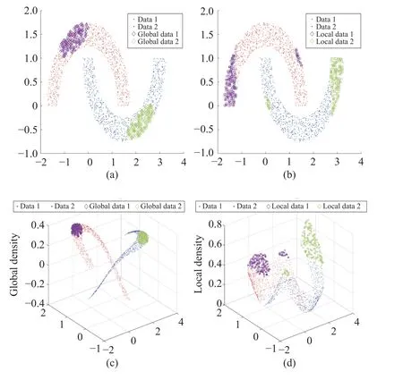
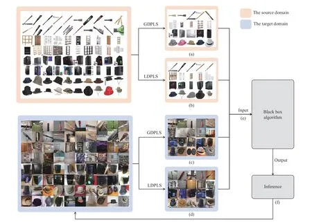
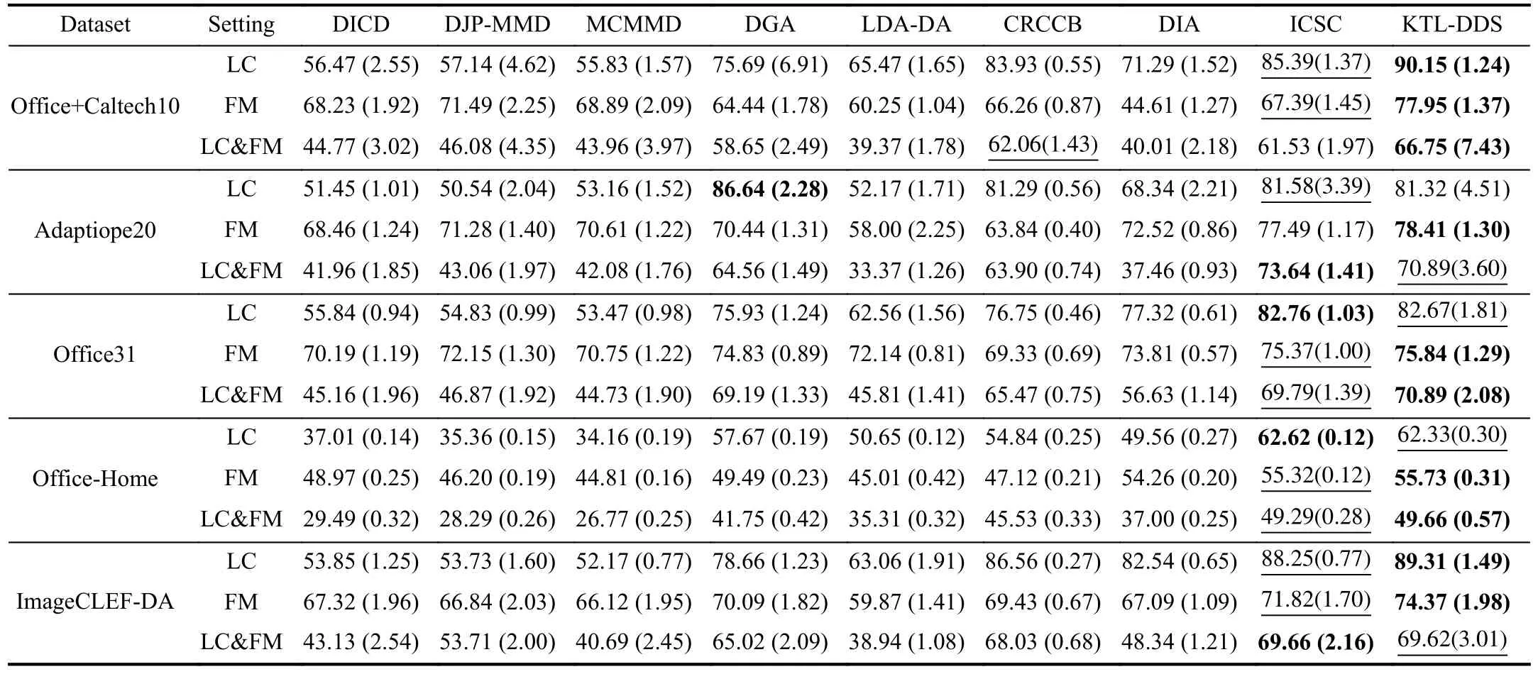
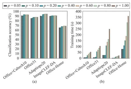
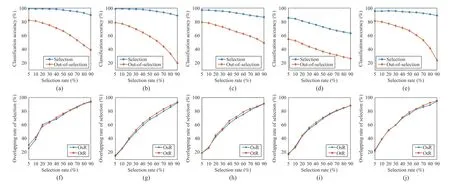
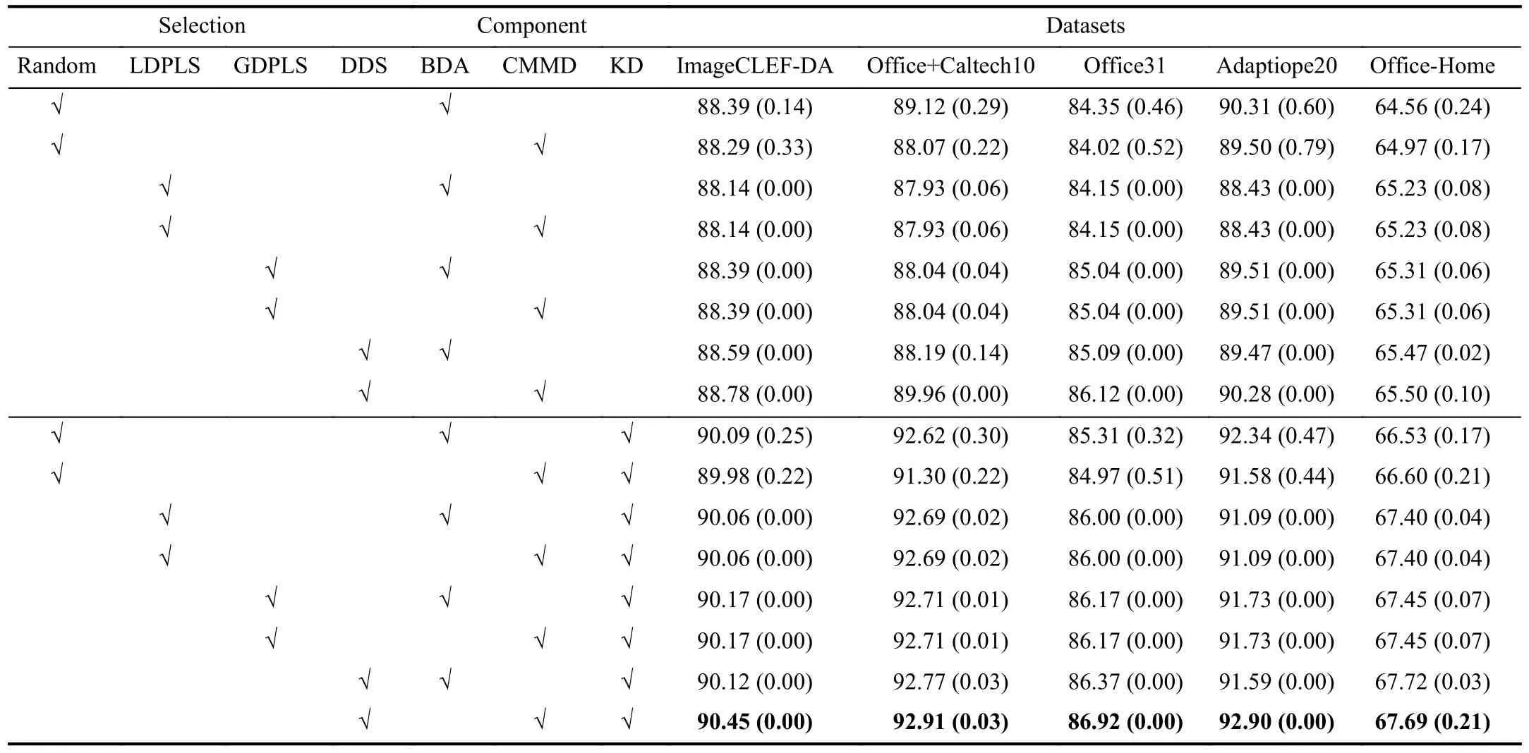
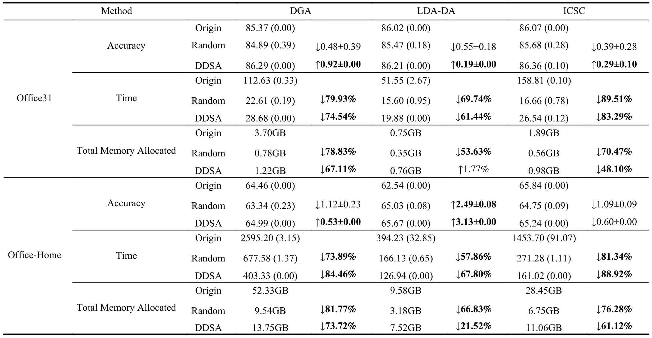
KTL-DDS consists of three parts: i) dual density sampling(DDS); ii) consistent maximum mean discrepancy (CMMD);and iii) knowledge dissemination (KD).Specifically, DDS jointly employs two sampling methods associated with different views: i) global density sampling, which extracts representative samples with the most common features and ii) local density sampling, which selects representative samples with critical boundary information.By measuring the global and local densities, four representative subsets with top⎿qtotaln」(0 Behind the effectiveness of KTL-DDS, mathematical analyses provide atheoretical foundation, showing that DDS needs to be executedonly once, which avoids repeated runs during iteration.Based on KTL-DDS, we further develop a lightweight framework dual density sampling approximation(DDSA).By using DDSA, the existing shallow algorithms can be easily transformed into those with low-computational-cost ones where encouraging performance is gained.As shown in the experiments later, DDSA reduces the training time of the algorithms and achieves performance close to that of the original algorithms.Hence, DDSA is expandable. The description of KTL-DDS is shown in Fig.1 and the main contributions are summarized as follows. 1) Dual density sampling (DDS) is proposed to select representative samples with high global or local densities.In doing so, the most common features (the global properties) and the marginal attributes (the local properties) are extracted for training jointly, which results in effective learning. 2) Consistent maximum mean discrepancy (CMMD) is introduced to reduce the differences of every pair of subsets among the four sampled subsets, which reduces the intra- and cross-domain risks for consistent knowledge learning. 3) Knowledge dissemination (KD) is employed to transfer confident and consistent knowledge from the representative samples (i.e., the samples with global and local properties) to the whole target domain.As a result, confident knowledge is learned from both the global and local perspectives. 4) Mathematical analysis is provided to show that DDS needs to run only once, which avoids repeated sampling during iteration and saves plenty of time. 5) A lightweight framework–dual density sampling approximation (DDSA)–is introduced for extensibility.DDSA accelerates the existing algorithms by an effective density sampling method DDS, and ensures that their performance is close to the original performance. By experiments, the effectiveness of KTL-DDS is verified by comparing eight shallow DA methods on five datasets in clean, label-noise, and feature-missing environments, and three deep learning methods on three popular datasets.In addition, tests on parameter sensitivity, convergence, and the validity are conducted. In this section, we first introduce the notations used in this paper and the problem of DA.Next, we review some maximum mean discrepancy (MMD)-based algorithms.Then, we analyze algorithms with low time complexity and their limitations.At last, we introduce some deep learning methods.At the end of each subsection, we describe the differences between KTL-DDS and the previous works. whereLis alossfunction,f(WT X,Ys)isaclassifier thatis jointlytrainedbythedomainfeaturesWT Xandthe semantic knowledgeYs, andfˆ(Xt) is a basic classifier trained on theoriginal feature spaceXt. TABLE I THE NOTATIONS Wanget al.propose an unified MMD algorithm called balanced distribution adaptation (BDA) [20].By BDA, the marginal and conditional distributions are balanced and jointly measured under the MMD metrics.Specifically, it aims to learn a projection matrixW∈Rm×d, so that wherex•,idenotes thei-th sample ofX•,X•crepresents the sample set consisting of samples from thec-th category inX•,anddenotes thei-th sample ofX•c. Although BDA can reduce the domain discrepancies effectively, it might suffer from insufficient representation and achieves limited performance.In light of this, Liet al.improve BDA by reducing intra-class dispersion and expanding inter-class dispersion [21].As a result, the discriminative features are explored and promising results are achieved.Unfortunately, since they neglect the negative effects caused by the class scatters, the algorithm might learn some redundant features.For this reason, Yang and Zhong introduce anℓ2,1constraint to penalize the projection matrix and achieve a sparse representation [22].To reduce the cross-domain risk,Duet al.embed the within-scatter into BDA and standardize the scatter metrics with the MMD metrics uniformly [23].Consequently, domain-invariant features are learned, crossdomain error is reduced, and increased performance is achieved. In order to reduce the joint probability distribution of two domains consistently, some variant methods are proposed[10], [24]–[26].Wanget al.dynamically adjust the relative importance of the marginal and conditional distributions, and learn a classifier with structural risk minimization (SRM) in the manifold subspace jointly.Wanget al.embed the label kernel into a DA algorithm, and propose a BDA-like framework called joint maximum mean discrepancy (JMMD) [26].JMMD jointly reweights and measures the joint probability of domains.Thus, great improvement is achieved.Based on the class-independence criteria, Zhang and Wu propose the discriminative joint probability maximum mean discrepancy(DJP-MMD) [10].At the class level, DJP-MMD aggregates similar samples and penalizes dissimilar samples, i.e., Since DJP-MMD uses the source label and target pseudo labelYˆt∈Rntto guide the model, incorrect pseudo-labeling might lead to the accumulation of errors.With this observation, Tenget al.introduce an adaptive adjustment strategy to progressively correct the mismatch during iteration [19].Liet al.propose a nested iterative optimization framework called progressive distribution alignment based on label correction(PDALC) [27].With PDALC, the confidence degrees of the target domain are measured in each iteration, while the distributions are progressively aligned according to the confidence level. By contrast, Xiaoet al.concatenate features and labels together, and optimize them simultaneously [25].Specifically,they aim to optimize whereW∈R(m+C)×dis the projection matrix,Y˜sandY˜tare the one-hotmatricesof source labelsYsand targetpseudolabelsYˆt,respectively,and [Xs;µY˜s]∈R(m+C)×nsis anoperation that concatenate the features and labels together. Although the above methods achieve good results, they are time-expensive (refer to Table III).For example, the time complexity of BDA isO(T(m3+mn2+m2n)) (Tis the iteration times,mis the inputting dimension, andnis the training size).Since the dimensionality reduction is verified experimentally to retain critical features [17], [28], we can easily ensurem≤n.Thereby, BDA requires computational timeO(Tmn2), which is highly related to the training scalen. Difference with the aforementioned MMD-based algorithms: As for the above MMD-based algorithms [10], [20],[25], [26], they mainly adopt MMD to reduce the discrepancies of the domains.In contrast, in this study, we propose CMMD to simultaneously address domain discrepancies and inconsistent knowledge caused by sampling.By using CMMD, both intra- and cross-domain risks are reduced and the convergence is significantly improved.Besides, a lightweight framework known as DDSA is introduced, which can be easily applied to the above MMD-based algorithms. There are some works focusing on efficient learning, such as optimal transport [29], [30], progressive learning [27], and subspace alignment [31], [32]. As for subspace learning, Sunet al.propose correlation alignment (CORAL) that aligns the second-order statistics of the distributions with time complexity O(m3+m2n) [31].In CORAL, the source samples are “whitened” and “re-colored”by two covariance metrics.Based on a basic classifier, Wanget al.propose a hyperparameter-free intra-domain programmingmethodcalledEasyTLwith timecomplexityO(Cn3s+C3n3t)[32], which alignstheclassification probabilityofthe domains.Luet al.propose substructural optimal transport(SOT) with time complexity O(T1Ln+T2L2) [30], whereT1andT2are the number of the iterations, andLis the number of clusters.SOT clusters the source and target samples, respectively, and learns an optimal transport scheme for these clusters.Wang and Breckon propose selective pseudo labeling(SPL) to progressively tag target samples [17]. Although the above-mentioned methods perform well, they still have some limitations that hinder their application.For example, due to the natural properties of optimal transport, it is difficult to combine SOT with other representation learning methods, such as manifold regularization [24], [33] and label regression [11].Generally, a mathematical derivation is needed to provide an optimal scheme under manifold (or label regression) constraints.As for EasyTL, it is highly dependent on the initial classifier.Thus, the constraints imposed on it may not yield improved performance.For SPL, its time complexity isO(T(m3+m2nspl+mn2spl)) (wherenspl=ns+qˆnt, andqˆis a variable that grows from 0 to 1).In its learning process,the tagging rateqˆ is increased with iterations, resulting in long iteration time (or long training periods). In contrast to the aforementioned algorithms [27],[29]–[32], a sampling method, namely DDS, is proposed to select samples with both global and local properties as the“reliable” ones for training.In this way, the efficiency of the algorithm and the quality of the selected samples are ensured simultaneously, and both global and local knowledge is learned at the same time.Due to the superiority of DDS, it is expected to impose growing constraints on it.In light of expandability, DDSA is further proposed as a general framework to improve the efficiency of conventional MMD-based algorithms, which is more general than the methods discussed above. In this subsection, we introduce some deep learning methods related to KTL-DDS.As for the other algorithms, interested readers can refer to surveys [8] and [34] to gain deep insight into them. Yanet al.propose weighted domain adaptation network(WDAN) that eases class weight bias using weighted maximum mean discrepancy (WMMD) [35].Huanget al.propose deep multi-representations adversarial learning (DMAL),which explores the pairwise relationships between domaininvariant, domain-specific, class-invariant, and class-specific features [36].By DMAL, some easily confused features between objects are removed, while representative features are exposed.Thus, the transferability and discriminability of the model are improved.In light of the time complexity, Zhuet al.introduce deep subdomain adaptation network (DSAN)[37], which measures the domain discrepancies by local maximum mean discrepancy (LMMD) between subdomains of the source and target domains.Similar to [30], DSAN divides the source and target domains into multiple subdomains and captures local discrepancies between subdomains.Since domain discrepancies are measured across many small-scale subdomains, DSAN converges quickly.Xiao and Zhang introduce dynamic weighted learning (DWL) [38].In DWL, the relative importance between distribution alignment and discrimination is dynamically measured.Since DWL adopts an effective weighting strategy, it achieves promising performance on a wide range of datasets.Different from DSAN, Jianget al.propose resource efficient domain adaptation (REDA) [12].In REDA, the learned knowledge is transferred progressively from the features extracted by a deep extractor to the ones by a shallow extractor.As the depth of the network increases, the network parameters gradually decrease.Hence, REDA reduces computational time effectively and achieves remarkable performance.Liet al.propose dynamic domain adaptation (DDA) [13].Before training, DDA computes the score of the target samples by averaging the prediction scores from all deep networks.Then, only a part of the high-confidence (high score) target samples is involved for training in each iteration.As a result, DDA reduces redundant calculations and achieves promising performance. However, due to the difference in the learning process between deep learning and shallow machine learning methods,the aforementioned deep learning strategies may not work well in shallow DA.Therefore, it is necessary to study an efficient shallow machine learning algorithm. Different from the above deep learning methods, we propose an effective sampling method DDS, and introduce CMMD to solve the inconsistencies caused by sampling.Compared with DSAN that reduces the local discrepancies between a number of small-scale subdomains [37], CMMD reduces the local discrepancies between the intra- and crossdomains generated by DDS.Different from DDA that selects some target samples in each iteration and learns the global knowledge only [13], KTL-DDS selects both the source and target samples before training, and learns both the global and local knowledge simultaneously.Different from the above deep learning strategies that require repeated sampling, mathematical evidence is provided in this study to show that the proposed method can avoid repeated sampling during iteration, which makes DDS effective and reliable. In this section, we present KTL-DDS in detail.First, we introduce global density peak landmark selection (GDPLS)and develop local density peak landmark selection (LDPLS).Then, we present DDS based on GDPLS and LDPLS.Based on DDS, we discuss the inconsistency caused by BDA and propose CMMD.Next, KD is given to transfer the confident knowledge from the representative target samples with global and local properties to the whole target samples.By doing so,the overall objective function, the optimization procedure, and the computational complexity are investigated.Based on KTL-DDS, an lightweight framework called DDSA is developed.At last, we mathematically show the consistency of the dual density sampling methods DDS and DDSA. In order to reduce the training scale, one promising way is to select ⎿qtotaln」 representative samples from the whole training set and use these samples for training [13], [17].This approach holds when it meets the following assumption. Assumption 1(Sampling Hypothesis):LetX∈Rm×nbe a sample set collected from one distributionPXandX˜ ∈Rm×n˜(n˜ where L(f1,f2) is a loss function that measures the performance discrepancies between classifiersf1andf2,f(X)denotes the classifier trained on feature spaceXandτis a threshold. Based on Assumption 1, the key to select samples is to detect representative samples.In recent clustering research,Chenget al.declare that the samples with high density might be the representative ones [39].However, owing to the discrepancies between domains, this view might work well in clustering, but fail in DA.In fact, in order to reduce domain discrepancies, the representative samples should have two properties: a) high density (high-confidence) [8], [17]; and b)high discrimination [10], [19], [40].Thanks to previous work[18], we can achieve this with Definitions 2 and 3. Definition 2(Global Density of DA[18]): LetX∈Rm×nbe the sample set with labelsY∈Rn, the global densitypg(xi) of each samplexiis defined as whereXc∈Rm×ncdenotes the sample set belonging to thec-th class,ncis the number of samples inXc, andz(xi,xj) isa radial basis function (RBF), i.e., withσbeing a hyper-parameter, which is fixed as 1 in the experiments. Definition 3(Global Density Peak Landmark Selection[18],GDPLS): LetX∈Rm×nbe a sample set with labelsY∈Rn.Global density peak landmark selection (GDPLS) is defined to extract a subsetXgfromXbyGg(X,q), whereGg(X,q)is a sampling function that selects the samples with top max⎿qn」 highest global densitypgby (6), 0 By Definitions 2 and 3, the global density meets the two conditions of the representative samples, i.e., high density and high discrimination.However, GDPLS might not be able to estimate the general features of domains accurately enough.As revealed by Figs.2(a)-2(d), GDPLS measures the global property of each sample, which helps to learn general classification knowledge.By contrast, samples with high local density might also be representative samples, since these samples compensate for the whole distribution carefully.They may not be the densest part of the distribution, but they give a better estimate of the classification boundary.With this in mind, we propose to use these samples by Definitions 4 and 5. Definition 4(Local Density of DA): LetX∈Rm×nbe a sample set with labelsY∈Rn, the local densitypl(xi) of the samplexiis defined as Fig.2.An example on the Double Moon distribution.The rhombus marker denotes the samples selected by global density, while the square marker denotes the samples selected by local density.(a) The results of the GDPLS on 2D space; (b) The results of LDPLS (the proposed one in this paper) on 2D space; (c) The results of GDPLS on 3D space, where the z-axis indicates the global density of the samples; and (d) The results of LDPLS (the proposed one in this paper) on 3D space, where the z-axis indicates the local density of the samples. whereNk(xi,X) is ak-nearest sample set formed byksamples closest toxiin the sample setX,z(xi,xj) is calculated by (7),andkis a hyper-parameter that determines the number of neighborhoods. Definition 5(Local Density Peak Landmark Selection,LDPLS): LetX∈Rm×nbe a sample set with labelsY∈Rn,local density peak landmark selection (LDPLS) is defined for extracting a subsetXlfromXbyGl(X,q), whereGl(X,q) is a sampling function that selects the samples with top max(⎿qn」,1) (0 Remark 1: It is worth noting that, whenk→∞, LDPLS is equal to GDPLS.In other words, GDPLS can be considered as a special case of LDPLS whenk→∞. Since both GDPLS and LDPLS are promising to select representative samples, we adopt them simultaneously.To avoid the influence caused by unbalanced categories, we define DDS by Definition 6, and select samples from each class. Definition 6(Dual Density Sampling,DDS): LetX∈Rm×nbe a sample set with labelsY∈Rn.Dual density sampling(DDS)is definedas selecting⎿qtotaln」(0 By introducing DDS, we select the samples with global densities and those with local densities from the source and target domains, respectively.In doing so, the samples with critical information are selected from two observation perspectives,while the noise samples might be filtered.As a result, both memory and time consumptions are reduced and promising performance is ensured. Another benefit brought by DDS is that it ensures the consistency of the sample selection, which is expected to avoid repeated selections during iteration.For simplicity, we mathematically analyze the consistency of LDPLS, and extend it to GDPLS and DDS. where L is a loss function, and ϵ is the error tolerance. Proof:Please refer to Appendix A.■ Corollary 1:Theorem 1 holds for GDPLS. Proof: Please refer to Appendix B.■ Corollary 2: Theorem 1 holds for DDS. Proof: Please refer to Appendix C.■ Based on the sampling hypothesis (Assumption 1), Theorem 1 shows that LDPLS (GDPLS and DDS) indeed maintains the relative density of categories from the original space to the projection subspace.Hence, we can adopt DDS before training and avoid repeated sample selection during iteration.As a result, fast convergence is guaranteed. In the next subsection, we utilize balanced distribution adaptation (BDA) [20] to overcome domain discrepancies,and then propose CMMD to tackle inconsistencies caused by BDA. By DDS, we denote the four subsets sampled from the source and target samples: i)Xs,g: the subset sampled fromXsby GDPLS; ii)Xs,l: the subset sampled fromXsby LDPLS; iii)Xt,g: the subset sampled fromXtby GDPLS; iv)Xt,l: the subset sampled fromXtby LDPLS. ˜Xs=[Xs,g,Xs,l] ˜Xt=[Xt,g,Xt,l] Denotes and.Then, one might adopt BDA to reduce the marginal and conditional distribution, so as to reduce the domain discrepancies and learn classification knowledge [20], i.e., Different from (2), (10) estimates the domain discrepancies by the sampling data, i.e.,X˜sandX˜t.As a result, the training scale is reduced. However, since GDPLS and LDPLS are related with different views, they may not cooperate well.Specifically, GDPLS captures the most common features of the categories, while LDPLS focuses more on the details of the samples.Hence,there might exist two inconsistencies that hinder the transfer learning of the knowledge: i)Intra-domain inconsistenciesthat is caused by the interaction of the samples with global and local densities in the same domain.In this case, it leads to two alignment risks ϵ(Xs,g,Xs,l) and ϵ (Xt,g,Xt,l); ii)Cross-domain inconsistenciesthat is caused by the measurement discrepancies in different domains.In this case, it leads to two cross-domain risks ϵ (Xs,g,Xt,l) and ϵ (Xs,l,Xt,g). To avoid inconsistencies and reduce the above risks, we introduce consistent maximum mean discrepancy (CMMD) by Definition 7. Definition 7(Consistent Maximum Mean Discrepancy,CMMD): CMMD is defined as a method that relaxes (10) so as to align the domain distributions and reduce the intra- and cross-domain inconsistencies.That is, By (11), we separately measure the discrepancies of every two subsets among the four subsets.By doing so, the consistency properties of the domains are guaranteed and improved performance is achieved.However, since (11) requires the calculation of MMD matrix six times, it is complicated and timeconsuming.In light of this, we develop Theorem 2 to simplify it. Theorem 2: (11) can be written as (12), i.e., where Proof: Please refer to Appendix D.■ By Theorem 2, we avoid the repeated computations of the MMD matrix.In doing so, (11) is integrated into a simpler form, which reduces computational time. With near observation, CMMD essentially reweights the relative importance of the selected samples and reduces both the alignment and cross-domain risks.By (11), the representative samples might be weighted twice by DDS, since these samples are the ones with both top ⎿qnc」 highest global and local densities in classc.In this case, the most common features are further emphasized, while the features from different observations are explored.The correction in the weights leads to more consistent and accurate results. By sampling local and global densities and using CMMD,the transfer knowledge is bridged.However, this might not be sufficient to establish the similar relationships between the sampling and target instances.Hence, we propagate knowledge from the selected target samples (i.e., the samples with global and local properties) to the whole target domain by a manifold regularization [41], i.e., Although (15) is a general manifold regularization term that preserves the local structure of the target domain, DDS is employed to extract the samples with global and local densities for knowledge learning.When imposing (15), the learned projection matrixWmight retain: a) the confident knowledge from samples with global and local properties; and b) the structural knowledge from the target domain itself.Hence,(15) ensures that the confident knowledge with global and local properties is transferred to the target domain, which results in promising performance. By combining (12) and (15), the objective function of KTLDDS to be optimized by eigenvalue-decomposition is as Algorithm 1 Knowledge Transfer Learning via Dual Density Sampling (KTL-DDS)Input: and : the source and target sample sets;Ys Xs Xt: the source label set;d: the dimensionality of the projection subspace;α,λ,δ,k,τ: the hyper-parameters;T: the number of iteration times;Output: W: the projection matrix;ˆYt Xt: the pseudo label set of target samples~T =0 Initialize ;ˆYt Xs Xt Initialize pseudo label by training and ;Gain , , and by Definition 6;Initialize Laplace matrix L by (15);~T Fig.3.A toy example explaining the framework of DDSA.(a) A part of source samples that are selected from the source domain by GDPLS; (b) A part of source samples that are selected from the source domain by LDPLS; (c) A part of target samples that are selected from the target domain by GDPLS; (d) A part of target samples that are selected from the target domain by LDPLS; (e) The selected source and target samples are used as input, and are trained by a black box algorithm; and (f) The labeled target samples (tagged by the black box algorithm) are used to propagate knowledge to the rest of the target samples. With the development of machine learning, many constraints are proposed, such as block diagonal representation(BDR) [42] and adaptive graph embedding (AGE) [43].However, it is tricky to improve the efficiency of a general algorithm, since they obey different assumptions. Fortunately, KTL-DDS can be easily extended as a lightweight framework to other MMD-based algorithms, which can effectively improve their efficiencies.Since the universal MMD-based algorithms do not necessarily use KD as a constraint, we transform KD into a Label Propagation term [44],which makes it independent of the training algorithm.For easy description, we call the extension method of KTL-DDS as dual density sampling approximation (DDSA).The pseudocodes of DDSA are shown in Algorithm 2, and a toy example that represents the framework of DDSA is given in Fig.3. As shown in Algorithm 2, we wrap an MMD-based algorithm as a black box one.In the training process, a part of the source and target samples are selected by DDS.Next, these selected samples are used for training.After that, KD is utilized to propagate the semantics of the selected samples to the rest of the samples in the target domain so as to learn the confident knowledge after DDS.As a result, the training is accelerated while promising performance is ensured. In this subsection, we analyze the computational complexity of KTL-DDS. First, the calculation of (15) might be time-consuming,since its time is O(m2nt+n2t).However, we can use a sparse matrix to store the Laplacian matrixLand make the time complexity less than O(m2nt+n2t).Second, because (15) does not require any prior knowledge in the optimization process, it can be pre-calculated and stored.During training, we load thetermΨ=XtLXtTfirst, and add Ψ to CMMD.In doing so, the time wastage in the cross-validation (or grid-search process) is avoided. TABLE II OVERVIEw OF THE DATASETS Algorithm 2 Dual Density Sampling Approximation (DDSA)Input: and : the source and target sample sets;Xs Xt: the source label set;f(Xs,Xt,Ys)Ys: an MMD-like algorithm;ξ=0.9 ξ: a propagation factor ( in the study);ˆYt Xt Output: : the pseudo label matrix for target samples Begin:ˆYt Xs Xt(1) Initialize pseudo label set by training a basic classifier on and ;Xs,g Xs,l Xt,g Xt,l(2) Gain , , , and by DDS (Definition 6);˜Xs=[Xs,g,Xs,l]∈Rmטns(3) Initialize ;˜Xt=[Xt,g,Xt,l]∈Rmטnt(4) Initialize ;˜Ys ˜Xs(5) Initialize as the source label set of ;f(˜Xs, ˜Xt,˜Ys) ˜Yt ∈R˜nt ˜Xt(6) Train , and gain the pseudo label set of by f;˜Rt ∈R˜nt×C ˜Yt(7) Initialize as a one-hot matrix of , where;˜S ∈R(nt+˜nt)×(nt+˜nt) Xt ˜Xt(8) Initialize similarity matrix between and by (16);Rt=(˜Rt)i,j=■■■■■■■1, ˜Yi= j 0, otherwise■■■■■■∈R(nt+˜nt)×C(9) Initialize ;˜Xt Xt Rt=(1-ζ)(I-ζ ˜S)-1Rt(10) Transfer the knowledge from to by ;ˆYt Xt ˆYt,i=argmax(Rt)i,:1 ≤i ≤nt■■■■■■0nt×C ˜Rt(11) Assign the pseudo label set of according to( );End Thus, we propose the following three feasible strategies to accelerate KTL-DDS: In this section, five popular datasets, as well as their experimental settings, are introduced.Then, the comparison experiments are done with other MMD-based algorithms.Finally,we analyze the parameter sensitivity, convergence and effectiveness of the KTL-DDS and DDSA. For easy reproduction, the code of KTL-DDS and DDSA are released at https://github.com/zzf495/KTL-DDS, while the code of other compared methods are available at https://github.com/zzf495/Re-implementations-of-SDA. In this paper, we use five popular datasets in DA for comparison, i.e., Office+Caltech10 [45], Office31 [46], Adaptiope20 [47], Office-Home [48], and ImageCLEF-DA [49].The overview of the datasets are shown in Table II. Office+Caltech10 [45] is a traditional dataset used in shallow transfer algorithms.In this dataset, there are four subdomains sampled from different platforms, including A (Amazon with 958 pictures), W (Webcam with 295 pictures), C(Caltech with 1123 pictures), and D (DSLR with 157 pictures).The pixels of each picture are different, and there are ten categories in each domain.In the experiments, we use the features extracted by [50].Twelve cross-domain tasks are selected for comparison, e.g., A →D, A →W, A →C,..., and C →W. Office31 [46] is composed of three sub-domains, i.e., Amazon (A) with 2817 samples, DSLR (D) with 498 samples, and Webcam (W) with 795 samples.The dataset contains 31 common categories.In the dataset, there are three types of pictures: a) online e-commerce pictures; b) high-resolution pictures; and c) low-resolution pictures.Different forms of sampling environments make the distribution of these images vary greatly.In the experiments, the features are extracted by [17].For comparison, six cross-domain tasks are conducted, i.e.,A →D, A →W,..., and W →D. Adaptiope [47] is a challenging dataset that includes more accurate labels than Office-Home [17].It contains three subdomains, including Product images (Pr), Real Life (Rl), and Synthetic (Syn).Each domain contains 12 300 images with different pixels.In the experiments, we use ResNet50 provided by [17], and extract the samples with 2048 features.Due to limitation of the device, the samples with the first 20 classes are used.To avoid ambiguity, we refer to this dataset as Adaptiope20.In the experiments, six tasks are used with2000 samples, i.e., P r →Rl, P r →Syn,...,and S yn →Rl. TABLE III THE AVERAGE (STD) TRAINING TIME OF DIFFERENT ALGORITHMS Office-Home [48] is a large dataset, which contains 65 kinds of different objects with 30 475 images.It has four subdomains: Art (Ar), Clipart (Cl), Product (Pr), and Real-World(Rw).These subdomains include 2427, 4365, 4439, and 4357 images, respectively.In the experiments, we use ResNet50 models to extract the features and conduct 12 cross-domain tasks, i.e., Ar → Cl, Ar → Pr,..., and Rw → Pr. ImageCLEF-DA [49] contains three sub-sample sets, i.e.,Caltech-256 (C), ImageNet ILSVRC2012 (I), and Pascal VOC2012 (P).Each domain contains 600 images with 2048 dimensions.In each domain, there are 20 categories, each with 30 images.Same as [17], we extract the images by ResNet50,and conduct six tasks for verification, i.e., C →I,C →P,...,andP →I. For comparison, we introduce eight promising shallow machine learning algorithms published recently, including DICD (2018) [21], DJP-MMD (2020) [10], MMCD (2020)[51], DGA (2020) [40], LDA-DA (2021) [25], CRCCB (2021)[52], DIA (2021) [53], and ICSC (2022) [19].The details of these methods can be found in Appendix E.Besides, three deep learning methods are compared on Office31, Office-Home, and ImageCLEF-DA, including TAT (2019) [54],DSAN (2020) [37], and ATM (2021) [55]. In the experiments, we follow the same protocol and adopt Principal Components Analysis (PCA) to reduce the dimensionality of the datasets to 512 dimensions [17].In the tables,we use “A →B” to denote that subdomain “A” is transferred to subdomain “B”.For observation purpose, the highest accuracy is shown in bold, while the second-highest accuracy is underlined. In the experiments, we fixT=10.Due to space limit, the setting of the compared methods can be found in Appendix E.For KTL-DDS, we fix the neighbor numberk=10, the regularization term λ=0.1, the knowledge dissemination term η=5 , the tradeoff weight µ=0.2, and the sampling rateq=0.2(i.e., 20% of samples are collected from GDPLS and LDPLS, respectively).Then, two hyper-parametersαandγare grid-searched in [0.1, 0.2, 0.3, 0.4, 0.5, 0.6, 0.7, 0.8, 0.9]. In this subsection, we compare the time complexity of different algorithms.Since deep learning methods take more time4, we only compare the shallow learning algorithms.In the experiments, we record the time when algorithms achieve their best results on the same machine with an Intel Core i9-9900K CPU@3.6Ghz and 32GB RAM.In Table III, result with * means that the corresponding algorithm achieves its best results using kernelization. As shown in Table III, KTL-DDS consumes the least time on four involved datasets, i.e., Office+Caltech10, Office31,Adaptiope20, and Office-Home.Specifically, KTL-DDS takes 7.83±1.00, 1 3.39±0.07, 1 7.63±2.41, and 1 17.49±11.72 seconds on Office+Caltech10, Office31, Adaptiope20, and Office-Home, respectively.Since the sample size of ImageCLEF-DA is small, KTL-DDS consumes 6.80±0.89 seconds, which takes 4.79±0.86 seconds longer than CRCCB. Moreover, DICD, DJP-MMD, MMCD, and ICSC project samples into the kernel space to guarantee transfer performance.Especially, DICD and MMCD require 4201.12±49.11 and 2499.50± 197.79 seconds to complete training on Office-Home, while KTL-DDS takes 117.49±11.72 seconds only.Compared with these MMD-based methods, we find that KTL-DDS is more efficient.Due to the strong consistency of the CMMD, KTL-DDS performs well without kernelization and achieves encouraging results with a suitable training time. Furthermore, we record the time consumption of each component of KTL-DDS as shown in Table IV.In the table,CMMD † denotes the method that solves CMMD and (17).From the results, we find that DDS takes up a significant amount of time, which means that it is essential to avoid repeated sampling during iteration.Due to the effectiveness of the proposed method shown by Theorem 1, we avoid repeated sampling, which makes KTL-DDS an effective algorithm. In the next subsection, we conduct the comparison experiments to verify the promising performance of KTL-DDS. In this subsection, we conduct the comparison experiments according to the experimental settings on the five datasets.4 Generally, the deep learning methods take at least 6 and 24 hours on Office31 and Office-Home with one GeForce RTX 3080, respectively.The results are recorded in Tables V-IX, where † denotes that it is a deep learning algorithm. TABLE IV THE AVERAGE (STD) TRAINING TIME OF EACH COMPONENT OF KTL-DDS TABLE V CLASSIFICATION ACCURACIES (%) ON OFFICE+CALTECH10 (DECAF) TABLE VI CLASSIFICATION ACCURACIES (%) ON ADAPTIOPE20 (RESNET50) Results on Office+Caltech10 (Decaf).From Table V,KTL-DDS achieves 92.91% classification accuracy, while ICSC achieves 91.34%.Next, we find that other MMD-based algorithms achieve an accuracy of around 89%, which is 3.91% less than KTL-DDS.Moreover, KTL-DDS shows the best performance on five out of 12 tasks. Results on Adaptiope20 (ResNet50).As shown in Table VI,KTL-DDS achieves the best performance on all six tasks, with 92.90% average accuracy.Since Adaptiope20 is challenging,the performance obtained by each algorithm varies widely.However, KTL-DDS achieves 1.92% improvement than LDA-DA, and has the best performance on five of six tasks. Results on Office31 (ResNet50).The results are shown in Table VII.On Office31, KTL-DDS achieves 86.87% accuracy, slightly higher (0.8%) than ICSC.On task A →D, KTLDDS achieves 92.17% accuracy, 4.22% higher than DGA.Compared with deep learning methods, KTL-DDS has inferior performance, which is 1.53%, 1.53%, and 2.96% lower than TAT, DSAN and ATM, respectively.However, KTLDDS consumes less time than these deep learning methods.For instance, ATM uses about 6 hours on Office31, while KTL-DDS spends about 13 seconds (as shown in Table IV).Thus, KTL-DDS can achieve an good performance with a significant time advantage on Office31. Results on Office-Home (ResNet50).As shown in Table VIII, compared with the shallow DA methods, KTL-DDS achieves advanced performance with 67.72% classification accuracy on Office-Home (ResNet50).Compared with deep learning methods, KTL-DDS achieves performance close to that of ATM and DSAN, and improved performance com-pared to TAT.As shown in Fig.5(a) later, whenq>0.2,KTL-DDS can achieve higher performance than whenq=0.2.Hence, KTL-DDS can clearly achieve a good result. TABLE VII CLASSIFICATION ACCURACIES (%) ON OFFICE31 (RESNET50) TABLE VIII CLASSIFICATION ACCURACIES (%) ON OFFICE-HOME (RESNET50) Results on ImageCLEF-DA (ResNet50).Since each domain contains 600 samples, the key to achieving good performance is the algorithm’s ability of extracting critical features.As shown in Table IX, KTL-DDS achieves 90.34%average accuracy, with the best performance on four out of six tasks.Moreover, KTL-DDS achieves 6.04%, 1.05%, and 1.44% improvement compared with DJP-MMD, ICSC, and TAT, respectively.Besides, KTL-DDS performs a bit better,0.14% and 0.38% better performance than DSAN and ATM,respectively. Based on the experimental results, we verify that KTL-DDS can address the resource-limited problems with great performance.In the experiments, KTL-DDS achieves encouraging performance while taking an appropriate amount of time on all involved datasets.Although only ⎿qtotaln」 representative samples are used, KTL-DDS still achieves great performance.These results confirm the validity of the DDS. To investigate the limitations of KTL-DDS, we conduct comparison experiments in three noise environments. 1) Label corruption (LC), which randomly changes 40% of labels to other labels; 2) Feature missing (FM), which replaces 40% of the features with the mean value; 3) Label corruption & feature missing (LC&FM), which adopts both 1) and 2) simultaneously. We run the experiments 20 times and record the average accuracies and standard deviations (std) as shown in Table X.From the results, we find that: 1) The results of DICD, DJP-MMD, MMCD, and LDA-DA are much worse than that of DGA, ICSC, and KTL-DDS in LC and LC&FM environments.Since ICSC improves DJPMMD on two effective strategies and DGA reduces the crossdomain risks by repulsive MMD, they achieve great performance.However, due to the limitations of MMD, the variant MMD methods (i.e., DICD, DJP-MMD, MMCD, and LDADA) gain limited performance.Thus, we conclude that the key to improve the transfer performance is to improve the discrimination of the model. 2) In the LC environment, KTL-DDS gains good results on Office+Caltech10 and ImageCLEF-DA, and achieves limited performance on Office31 and Adaptiope20.Due to the effectiveness of the consistent properties, KTL-DDS always maintains better results than the conventional MMD methods (i.e.,DICD, DJP-MMD, MMCD, and DIA).However, since DDS leverages semantics to select samples, the noise samples mayhinder DDS and affect its performance. TABLE IX CLASSIFICATION ACCURACIES (%) ON IMAGECLEF-DA (RESNET50) TABLE X COMPARISON ExPERIMENTS UNDER NOISE ENVIRONMENT ON FIVE DATASETS 3) In the FM environment, KTL-DDS outperforms all compared algorithms.Especially, KTL-DDS achieves 6.46%,0.92%, 0.47%, 0.41%, and 2.55% improvements compared to the second-best algorithm on Office+Caltech10, Adaptiope20,Office31, Office-Home, and ImageCLEF-DA, respectively.The results confirm the effectiveness of the DDS and CMMD. 4) In the LC&FM environment, KTL-DDS achieves similar classification results as ICSC.However, the results of KTLDDS are more volatile, which is likely due to the joint effect of noise and missing data. In summary, since DDS requires some semantic information, the noise in the datasets might impact performance.As revealed by the experiments, KTL-DDS can achieve a suitable result in noisy environments, which verify its effectiveness. The sensitivity of parametersαandγ.The results are shown in Figs.4(a)-4(e).On Office+Caltech10, KTL-DDS achieves promising performance when 0.5 ≤α,γ ≤0.7; on Adaptiope20, KTL-DDS gains great classification effect when α=γ=0.4; on Office31, KTL-DDS gains the best performance when α =0.3 and γ =0.6; on Office-Home, KTL-DDS achieves good performance when γ=0.9 and β=0.7; on ImageCLEF-DA, KTL-DDS acquires promising results when α=0.2 and γ ≤0.6.Therefore, we prefer to searchαin [0.3,0.4, 0.5, 0.6] andγin [0.4, 0.5, 0.6, 0.7, 0.8, 0.9], and tune them carefully. The sensitivity of parameterq.We verify the effect of the training rateqon DDS, as shown in Figs.5(a) and 5(b).Whenq≤0.1, KTL-DDS might not work well on the datasets.We conjecture that this might be due to the small sample scale.Whenq≥0.2, the classification performance is close on different training scales.Besides, the training time of KTL-DDS increases with the increase ofq.Whenq=0.2, KTL-DDS achieves encouraging performance with appropriate time consumption. Fig.4.The sensitivity of hyper-parameters with respect to α and γ.(a) The results of task C →W on Office+Caltech10 (Decaf); (b) The results of task D →W on Office31 (ResNet50); (c) The results of task R l →Syn on Adaptiope20 (ResNet50); (d) The results of task C →P on ImageCLEF-DA (ResNet50);and (e) The results of task A r →Cl on Office-Home (ResNet50). Fig.5.The sensitivity of hyper-parameters with respect to q.(a) The classification results of KTL-DDS with respect to q on different datasets; and (b)The training time of KTL-DDS with respect to q on different datasets.The xaxis (from left to right) presents the results on Office+Caltech10, Office31,Adaptiope20, ImageCLEF-DA, and Office-Home, respectively.The y-axis in the sub-figures (a) and (b) denotes the classification accuracy and the training time, respectively. For a deep study, we record the accuracy of the selection and the out-of-selection, and the overlapping rate under differentqon different datasets.As shown in Figs.6(a)-6(e), the representative samples selected by DDS are more reliable than the out-of-selection samples.The results demonstrate that DDS can achieve similar performance when the training scale is small.As shown in Figs.6(f)-6(j), whenq=0.2, about 40%of the selected samples overlap.With the increase ofq, the overlapping rate increases as well.However, their performance is close.By contrast, whenq≤0.1, only a small number of samples overlap.Since the overlapping samples are the intersection of two views, they might contain more reliable information.From the experiments, we conjecture that these overlapping samples are the key to achieving promising performance on the small-scale dataset.Hence, we can letq≥0.2, and find a great compromise between selection rate and overlapping rate. The sensitivity of parameterη.As shown in Fig.7(a),KTL-DDS achieves stable performance on Office31, Adaptiope20, Office-Hom, and ImageCLEF-DA whenηchanges.On Office+Caltech10, KTL-DDS achieves advanced performance when η ≥5.Sinceηcontrols the weight of the structure, we prefer to fix it as η =5. The sensitivity of parameterλ.λis a regularization term which controls the extent of change.As shown in Fig.7(b),when 0.02 ≤λ ≤0.1, KTL-DDS gains promising performance on the five datasets.With this observation, we suggest fixing λ=0.1. The sensitivity of parameterk.As shown in Fig.7(c),KTL-DDS achieves stable performance regardless of the value ofk.Sincekcontrols the number of the nearest neighbors, it is insensitive in the experiments.Therefore, we can fixk=10and adjust other hyper-parameters. The convergence of KTL-DDS.The results are plotted in Fig.7(d).From the results, we find that KTL-DDS converges fast (T≤2 ).WhenT>2, the values of the objective function with respect to KTL-DDS remain stable.This phenomenon indicates that CMMD leads to strong consistency, and KTLDDS has good convergence properties. In this subsection, we verify the effectiveness of KTL-DDS by selecting following five components: 1) Random, which selects⎿qtotalnc」 samples from each classcin the source and target domains randomly; 2) DDS, which selects about⎿qtotalnc」 samples from each classcaccording to their global and local densities; 3) BDA, a basic model in DA, which is the specific case of CMMD whenq=1. 4) CMMD, which reweights the samples with global and local density.It is worth noting that, when using LDPLS (or GDPLS) only, CMMD is equivalent to BDA. 5) KD, which propagates the knowledge from the samples with global and local properties to the whole target domain by manifold assumption. In the experiments, we repeat the algorithm 20 times and record their classification accuracy.The experimental results are shown in Table XI.From the results, KTL-DDS achieves the best results, with 90.45±0.00%, 92.91±0.03%,86.92±0.00%, 92.90±0.00%, and 67.69±0.21% average accuracies on ImageCLEF-DA, Office+Caltech10, Office31, Adaptiope20,and Office-Home, respectively.Based on Table XI, we draw the following conclusions: 1) DDS helps to collect the representative samples.When using BDA, the results of DDS are more stable than that of“Random”.When using CMMD (+KD), DDS achieves a better performance than “Random” on all datasets.From the results, we find that DDS is stable and helps to achieve promising results. 2) CMMD helps to obtain consistent and stable results.On Office+Caltech10, CMMD achieves 1.77±0.14% average accuracy improvement than BDA.When adopting DDS,CMMD can obtain more promising performance than BDA.With the help of KD, CMMD further achieves better results and gains five best performance on all datasets.These results confirm the validity of CMMD. Fig.6.Statistics for different selection rate q under different datasets, where x-axis represents the selection rate for selecting samples from GDPLS and LDPLS, respectively.(a)–(e) denote the accuracies of selected and unselected samples under different selection rate q on Office+Caltech10, Adaptiope20,Office31, Office-Home, and ImageCLEF-DA, respectively; (e) and (f) present the proportions of overlapping samples to the selected samples on Office+Caltech10, Adaptiope20, Office31, Office-Home, and ImageCLEF-DA, respectively, where “OsR” denotes the proportion of overlapping samples to the selected samples in the source domain and “OtR” denotes those in the target domain. Fig.7.The sensitivity of hyper-parameters with respect to η, λ, k, and T.(a) The sensitivity of hyper-parameter with respect to η; (b) The sensitivity of hyperparameter with respect to λ; (c) The sensitivity of hyper-parameter with respect to k; and (d) The convergence of different tasks with the number of iterations T =10. In this subsection, we verify the effectiveness of DDSA.We conduct experiments for six MMD-based algorithms, including DICD, DJP-MMD, MMCD, DGA, LDA-DA, and ICSC on two popular datasets Office31 and Office-Home.First, we adopt DDSA to select about 20% samples according to GDPLS and LDPLS, respectively.Next, we use these selected samples as input for each involved DA method.Then, the selected samples are predicted and KD is utilized to propagate these samples to the rest of the samples that are not involved in the training.For fairness, the performance of the random strategy is used to compare.Finally, we record the classification accuracy as well as the training time in Tables XII and XIII.In the tables, we denote a) “Origin” that all of the samples are used for training; b) “Random” that the training samples are selected randomly from the datasets; c) “DDSA” that the training samples are selected by DDS; d) “↑ ” that the results are higher than “Origin”; and e) “ ↓” that the results are lower than “Origin”. As shown in Tables XII and XIII, using a selection strategy can significantly reduce training time.When DDSA is adopted, at least 70% of the training time is saved on Office-Home.Notably, we reduce the time of MMCD from about 2499.50 seconds to 167.02 seconds, and the time of DICD from about 4201.12 seconds to 546.92 seconds.Although only a portion of the data is used (about 30–40% in the experiments), DDSA achieves improved performance for six involved algorithms on Office31, and close performance on Office-Home.As for DJP-MMD, DDSA improves 2.13% and 6.75% classification accuracies on Office31 and Office-Home,respectively.When the random strategy achieves inferior performance (e.g., LDA-DA and ICSC on Office31, and DGA on Office-Home), the results obtained by DDSA are similar to the experiments with full data.The results show that DDSA is expected to replace the random strategy to save training time and achieve encouraging performance. To further illustrate the difference between DDSA and theand Office31+Office-Home are 8.21×10⁻³⁰, 6.69×10⁻²⁷, and 1.80×10-54, respectively.Since all thep-values are less than random strategy, we perform a significance analysis for them.We assume that there is no significant difference between DDSA and the random strategy at a 5% significance level5The null hypothesis.As shown in Table XIV, thep-values of Office31, Office-Home,0.05, thenull hypothesisis rejected at the 5% significance level.Hence, DDSA and the random strategy are significantly different. TABLE XI ABLATION ExPERIMENTS ON DIFFERENT DATASETS TABLE XII THE RESULTS OF DDSA/RANDOM + DICD/DJP-MMD/MMCD ON OFFICE31 AND OFFICE-HOME In summary, we show that DDSA achieves encouraging performance by using less samples.The experimental results demonstrate that DDSA can be used in the resource-limited scenarios, which saves a lot of time for training large-scale data. TABLE XIII THE RESULTS OF DDSA/RANDOM + DGA/LDA-DA/ICSC ON OFFICE31 AND OFFICE-HOME TABLE XIV THE P-VALUE ON OFFICE31 AND OFFICE-HOME In order to achieve close performance by sampling, we develop an effective method called knowledge transfer learning via dual density sampling (KTL-DDS) in the study.KTLDDS is composed of three components: 1) Dual density sampling (DDS); 2) Consistent maximum mean discrepancy(CMMD); and 3) Knowledge dissemination (KD).To reduce the training time, DDS selects representative samples that are composed of top ⎿qtotaln」 highest global or local densities from GDPLS and LDPLS, respectively.Then, CMMD narrows the differences of every two subset among the four representative subsets extracted by DDS, and reduces the intraand cross-domain risks simultaneously.To further convey confident knowledge from the representative samples (the global and local instances) to the whole target domain, KD employs a manifold assumption to explore the structure information of the target domain.By using KTL-DDS, consistent and confident knowledge is learned and advanced performance is ensured in a short time. A mathematical analysis is given to show that DDS can be executed only once and achieve close performance.By extending KTL-DDS, a general framework namely dual density sampling approximation (DDSA) is further proposed.DDSA accelerates the existing MMD-based algorithm and retains their promising performance with low-time complexity.The experiments conducted on five datasets in clean, label corruption (LC), feature missing (FM), and LC&FM verify the effectiveness of the KTL-DDS, and experiments on Office31 and Office-Home verify the promising application of DDSA. Limitations and future work: Despite the good results achieved by KTL-DDS and DDSA, there are still some issues that require in-depth study: 1)The application of DDSA to deep learning requires insightful investigation.Due to the impact of batch training,Theorem 1 (and DDSA) cannot directly apply to deep DA methods.However, we can still use DDSA to facilitate the training of deep DA methods.For example, we can add a small portion of the data sampled by DDS to the batch training so as to accelerate the convergence of deep learning algorithms and improve its performance.Unfortunately, due to space limit, we only extend DDSA to the shallow approaches and have not yet applied it to the deep DA methods, which makes this promising attempt a future work. 2)The threshold k w.r.t the density needs in-depth study.In Definition 4, we use a uniform hyperparameterkto estimate the local density of samples.However, the number of categories in the dataset may be unbalanced in practice.In this case, a fixedkmay lead to an incorrect local density estimation, and limit the performance of DDS.Thus, an in-depth discussion ofkis needed. Proof: First, we introduce the following symbols: 1)Xout=XXˆ is the out-of-selection sample set; 2) The matrixXwith superscriptcindicates the set of samples belonging to thec-th category inX; Proof: Given the same conditions as in Theorem 1, similar to (21) and (22), we can get and Obviously, by bringing (27) and (28) into (6) and (7),Corollary 1 holds.■ Proof: Based on Theorem 1 and Corollary 1, by tuning the weights of samples with respect to LDPLS and GDPLS,Corollary 2 also holds for DDS (or DDSA) with different estimation error ∆error. Proof: The proof is done by deriving the marginal distribution, which can also be applied to the conditional distribution. and which indicates Similarly, we can get whereXl→g,l=[Xs,l,Xt,g,Xt,l], and In doing so, the first four terms of (11) are simplified to calculate the two marginal matrices as (33) and (35). Furthermore, if we combine γM(W,Xs,g,Xs,l) into (32) and(34), a weightγis introduced to balance the relative importance ofXs,gandXs,l.Therefore, (32) and (34) can be transformed into (36). whereXg,l→g,l=[Xs,g,Xs,l,Xt,g,Xt,l] and From (37), we find thatXs,gandXs,lare balanced by a hyper-parameterγ, whileXt,gandXt,lare balanced byαandβ,respectively. For the sake of balance, we set α +β=1 to further simplify the formula, i.e., By combiningM(W,Xt,g,Xt,l) and (38), the parameter inM(W,Xt,g,Xt,l)is no longer controlled byγ, but byα(orβ).Therefore, we can get the same form of (12) with marginal matrixMˆ0=Q0(Q0)T. Similarly, by the same derivation as above, we can getMˆc=Qc(Qc)T, which completes the proof.■ Domain Invariant and Class Discriminative (2018,DICD) [21] simultaneously reduces the marginal and conditional distributions.Moreover, the within-class and betweenclass scatters are employed to learn discriminative knowledge.In the experiments, the regularization parameterβis searched in [0.1, 1], whileρis searched in [0.01, 0.02, 0.05, 0.1, 0.2,0.5, 1, 2, 5, 10]. Discriminative Joint Probability Maximum Mean Discrepancy (2020, DJP-MMD) [10] is a variant method of MMD.Based on the independence assumption of categories,DJP-MMD narrows the distances between the same centroids and enlarges the distances of different centroids in two domains.In the experiments, the regularization parameterλis searched in [0.1, 1], while the trade-off parameterμis gridsearched in [0.1, 0.2, 0.3, 0.4, 0.5, 0.6, 0.7, 0.8, 0.9]. Maximum Mean and Covariance Discrepancy (2020,MMCD) [51] jointly use MMD and maximum covariance discrepancy (MCD).Since both one-order and second-order statistics are used, MMCD achieves improved performance.In the experiments, the trade-off parametersβandλare gridsearched in [1 0-5, 1 0-4, 1 0-3, 1 0-2, 1 0-1, 1, 10, 102, 103, 104,105]. Discriminative and Geometry-Aware (2020, DGA) [40]jointly reduces marginal, conditional, and cross-domain distributions.In DGA, two repulsive terms are proposed to reduce the cross-domain risks, while the label smoothness is used to guarantee the consistency of the classification.In the experiments, the regularization parameterλis fixed as 0.1, and the balance parameterαis given as, whereμis searched in[0.01, 0.02, 0.05, 0.1, 0.2, 0.5, 1, 2, 5, 10]. Label Disentangled Analysis (2021, LDA-DA) [25] concatenates the features and the labels into an unified framework.In LDA-DA, the global properties of the features and the semantics are jointly explored.In the experiments, the regularization parameterλand the tradeoff parameterμare gridsearched in [0.1, 0.2, 0.3, 0.4, 0.5, 0.6, 0.7, 0.8, 0.9, 1.0, 1.1,1.2, 1.3, 1.4, 1.5, 1.6, 1.7, 1.8, 1.9, 2.0]. Collaborative Representation with Curriculum Classifier Boosting (2021, CRCCB) [52] is an effective algorithm,which reconstructs the source samples and “reliable” target samples progressively.In the experiments, we tune the number of the iterationsTin [5, 6, 7, 8, 9, 10]. Discriminative Invariant Alignment (2021, DIA) [53] is a coupled projection learning algorithm, which embeds withinand between-class scatters into the learning framework.In the experiments, we fix α=1, and grid-searchβin [0.01, 0.02,0.05, 0.1, 0.2], andμin [0.005, 0.01, 0.02, 0.05]. Incremental Confidence Samples into Classification(2022, ICSC) [19] improves DJP-MMD by introducing adaptive adjustment and progressively tagging strategies.During iteration, the target samples are tagged progressively according to the classification confidence, while the distributions are adaptively weighted.In the experiments, the regularization parameterλis searched in [0.1, 1], while the trade-off parameterμis searched in [0.1, 0.2, 0.3, 0.4, 0.5, 0.6, 0.7, 0.8, 0.9].II.RELATED WORk
A. Notations and the Problem of DA

B. MMD-Based Algorithms
C. Algorithms for Fast Training or Inference
D. Deep Learning Algorithms
III.PROPOSED METHOD
A. Dual Density Sampling

B. Consistent Maximum Mean Discrepancy

C. Knowledge Dissemination
D. Optimization


E. Extending to Other General Algorithm
F. Computational Complexity


IV.ExPERIMENTS
A. Involved Datasets

B. Compared Methods
C. Experimental Setting
D. Training Time of Different Algorithms
E. Comparison Experiments


F. Experiments under Noise

G. Parameter Sensitivity and Convergence Analysis

H. Ablation Study

I. Experiments of DDSA


V.CONCLUSION
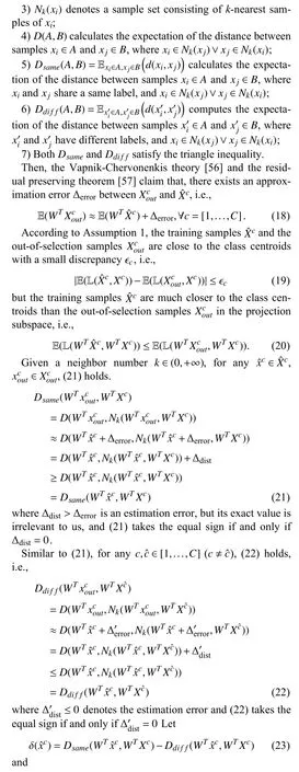
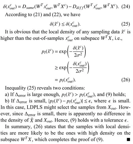
APPENDIx A PROOF OF THEOREM 1
APPENDIx B PROOF OF COROLLARY 1
APPENDIx C PROOF OF COROLLARY 2
APPENDIx D PROOF OF THEOREM 2
APPENDIx E INTRODUCTION AND ExPERIMENTAL SETTING OF COMPARISON METHODS
杂志排行
IEEE/CAA Journal of Automatica Sinica的其它文章
- A Game Theoretic Approach for a Minimal Secure Dominating Set
- Subspace Identification for Closed-Loop Systems With Unknown Deterministic Disturbances
- Magnetic Field-Based Reward Shaping for Goal-Conditioned Reinforcement Learning
- Multi-Blockchain Based Data Trading Markets With Novel Pricing Mechanisms
- GenAI4Sustainability: GPT and Its Potentials For Achieving UN’s Sustainable Development Goals
- Resilient Event-Triggered Control of Connected Automated Vehicles Under Cyber Attacks
