A dynamic fusion path planning algorithm for mobile robots incorporating improved IB-RRT∗and deep reinforcement learning①

LIU Andong(刘安东),ZHANG Baixin,CUI Qi,ZHANG Dan,NI Hongjie②

(College of Information Engineering,Zhejiang University of Technology,Hangzhou 310023,P.R.China)

Abstract

Key words:mobile robot,improved IB-RRT∗algorithm,deep reinforcement learning(DRL),real-time dynamic obstacle avoidance

0 Introduction

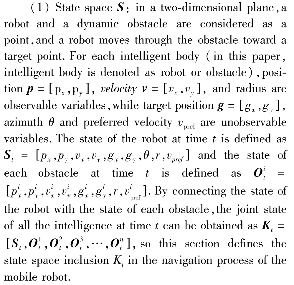
With the rapid development of robotics technology,mobile robots have become increasingly prevalent in industries such as military,medical,logistics,and service fields.This widespread use of mobile robots is largely attributed to the development of autonomous navigation technology.The purpose of path planning[1]is to plan a safe path to avoid obstacles in a specific working environment according to certain evaluation criteria,such as time and distance.According to the surrounding environment information of mobile robots,path planning method can be divided into two categories: global path planning with a known environment[2-3]and local path planning with an unknown environment[4-5].Traditional global path planning algorithms include the graphics methods,such as the visibility graph method[6-7],graph search-based algorithms like A∗algorithm[8-9],and random sampling planning algorithms like RRT∗algorithm[10].On the other hand,local path planning based on sensor information encompasses methods such as the artificial potential field method[11],the dynamic window method[12],and deep reinforcement learning (DRL) methods[13].

In complex environments, the visibility graph method requires reconstructing the map when the search conditions change,the node calculation of the A∗algorithm is large and the planning efficiency is low,so it is not suitable for use.The RRT∗algorithm boasts asymptotic optimality and can efficiently search the entire solution space,making it suitable for complex environments.However,the drawback of RRT∗is also obvious: after quickly finding the initial path,the algorithm needs to keep optimizing as the sampling points keep increasing,which means that a lot of time needs to be spent on the convergence of the algorithm.Ref.[14] proposed a bidirectional search algorithm by generating two search trees at the starting point and the target point in parallel to improve node expansion efficiency and speed up convergence.However,the algorithm cannot avoid a large number of invalid sampling in the sampling space,resulting in a long search time.To deal with invalid sampling in the sampling space,the informed-RRT∗algorithm has been proposed in Ref.[15] by using a state subset to optimize the sampling space,which obtains the optimal path,but the search time of this algorithm is still long.Ref.[16]combined the bidirectional search with the heuristic function of intelligent sample insertion for making the algorithm converge rapidly,but the planned path was relatively long.Furthermore,these algorithms are limited in their ability to handle unknown obstacles and dynamic obstacle avoidance.

The basic idea of the artificial potential field method[17]is to concretize the influence of targets and obstacles on the movement of the robot into an artificial potential field.The potential energy at the target is low and the potential energy at the obstacle is high.This potential difference generates the gravitational force of the target on the robot and the repulsive force of the obstacle on the robot,whose combined force controls the robot to move towards the target point along the negative gradient direction of the potential field.However,this method does not account for the robot's dynamic constraints and can result in a local optimum problem.

The dynamic window method[18]seeks the optimal control speed in the speed space of the mobile robot under the dynamic constraints,which can realize realtime path planning and dynamic obstacle avoidance.However,this method cannot obtain the globally optimal path and easily falls into the local minima problem.In addition,the above-mentioned traditional local planning algorithms all prevent collisions or define functions to ensure safety through passive reactions,resulting in a robot that cannot assess the impact of current actions on the system in the long run and has a slow response speed.DRL[19]has become a popular research topic since AlphaGo's success in defeating a human Go champion.DRL is an adaptive dynamic programming method based on the Markov decision process and can improve a robot's decision-making ability by providing optimal decisions based on data.Ref.[20] applied DRL to a mobile robot exploring an indoor environment by inputting the original depth images into a deep Q-network (DQN) to obtain movement commands.The method significantly improved the cognitive ability of the mobile robot compared to the supervised approach.In Ref.[21],an end-to-end path planning method has been proposed for solving the problem of relying too much on map information in the traditional human planning framework by using radar and camera information and combined with the dueling double DQN priority experience recall (D3QN PER) algorithm in deep reinforcement learning to make action commands directly for a mobile robot,but the method will make the robot plan a longer path,increasing the search time and reducing the efficiency of navigation.Ref.[22]used DRL to model human-robot interaction for crowd-aware navigation in simulation,but when the target location is far away,it makes the robot go around and increases the navigation time.

This paper presents a novel dynamic path planning algorithm that combines the improved IB-RRT∗with deep reinforcement learning.Firstly,the improved IB-RRT∗algorithm is utilized to rapidly plan the globally optimal path,while LIDAR-acquired information about the surrounding environment is fed into the trained DRL model to output action commands so that the robot can have autonomous decision-making capability and thus achieve local dynamic obstacle avoidance in unstructured environments.The effectiveness of the improved IB-RRT∗is demonstrated through simulations conducted in Matlab, and compared with Bi-RRT∗,Informed-RRT∗,and IB-RRT∗algorithms.Furthermore,a mobile robot navigation experiment is given to validate the proposed fusion algorithm in a realistic environment with random dynamic obstacles.

1 Global path planning based on improved IB-RRT∗algorithm

IB-RRT∗is a non-greedy trees connection global path planning algorithm,but it has the disadvantages of more search nodes and longer path length.In this section, the IB-RRT∗algorithm is improved by using probabilistic central circle target bias,double elliptical sampling,and intelligent sample insertion to reduce the number of useless nodes generated by sampling and increase the convergence speed.The details of these enhancements are further discussed in the following subsections.

1.1 Probabilistic central circle target bias

Although random sampling can avoid the random tree expansion trapped in the local optimal solution,there will be the problem of the too-long initial path,resulting in too large ellipse sampling space and slow convergence of the algorithm.Therefore,a probabilistic central circle target biasing strategy is introduced for IB-RRT∗to make the random tree search toward the central circle target as much as possible to speed up finding the initial path.The target biasing strategy is expressed as

whereXcentercircleis a circle with the central coordinates of the starting point and target point as the central of the circle and radius asR,and when the random probability is greater thanPsetthen it is expanded to the central circle, otherwise,the points are generated randomly on the map.An illustration example of probability central circle target bias is shown in Fig.1.

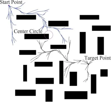
Fig.1 Probability central circle target bias

It can be seen from Fig.1 that the implementation of probabilistic central circle target bias has a significant impact on the acceleration of bidirectional random tree connection.The random point generation process is not impacted by obstacles located at the central point,thus enabling the probabilistic central bias to both prevent the occurrence of local optima and expedite the time required to find the initial path.

1.2 Double elliptic subset sampling domain

In order to reduce useless sampling space,The elliptic subset sampling domain method[15]is introduced in this section to quickly find the optimal path due to its little dependence on the dimension of the planning problem and the current state space.

The elliptic subset sampling domainXf^is an ellipse with the initial statexsand the target statexgas the focal points.It is known that the sampling area range depends on the initial statexsand the target statexg.The parameters of the considered ellipse are defined thatcmin= ‖xg-xs‖is the focal length,the current path costcbestis the long axis of the ellipse,is the short axis of the ellipse, andXis the state space,as shown in Fig 2.Therefore,the state in the ellipse sampling domain is given as follows:

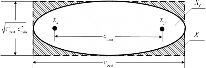
Fig.2 Elliptic subset sampling domain

Based on the elliptic subset sampling domain,the uniform sampling samplexellipse～ U(Xellipse)can be obtained by converting the uniformly distributed samples in the unit circlexball～ U(Xball),i.e.

wherexballis the uniformly sampled point in the unit circle,xcentreis the center point of the ellipse,andLis a transformation matrix withLLT=S,andSis the diagonal matrix obtained by decomposing the hypelliosoid matrix.

Substituting Eq.(4) intoLLT=S,the transformation matrix can be obtained as

where,diag ·{ }is a diagonal matrix.

The rotation from the elliptical to the world coordinate system can be viewed as a Wahba problem[23]for solving.Thus,the rotation matrix is defined as

wheredet·( )is a diagonal matrixUandVcan be obtained from the rotation matrixMby singular value decomposition,the rotation matrix is defined as

Therefore,the elliptic subset can be obtained by transforming, rotating, and translating the uniformly sample points.Sampling point is given as follows

The specific algorithm process is shown in Algorithm 1.

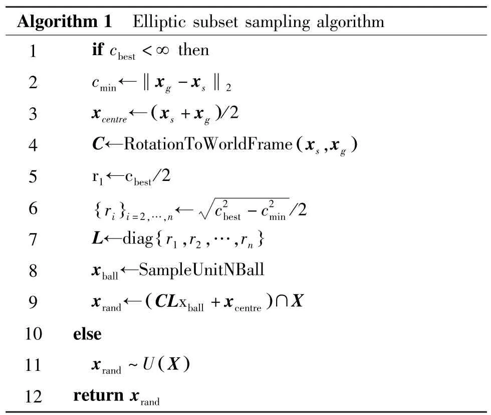
Algorithm 1 Elliptic subset sampling algorithm 1 if cbest <∞then 2 cmin←‖xg -xs‖2 3 xcentre← xs +xg ( )/2 4 C←RotationToWorldFrame xs,xg ( )5 r1←cbest/2 6 {ri }i=2,…,n← c2 best -c2/2 7 L←diag r1,r2,…,rn min {}8 xball←SampleUnitNBall 9 xrand← CLxball +xcentre ()∩X 10 else 11 xrand ～U (X )12 return xrand

The double elliptic subset sampling domain,depicted in Fig.3,uses the connection point as the focal point for the first ellipse and the starting point as the focal point for the second ellipse.This design results in further reduction of redundant sampling space compared to traditional ellipse sampling.

Fig.3 Double elliptic subset sampling domain

1.3 Improved IB-RRT∗algorithm

The IB-RRT∗algorithm implements bidirectional trees and intelligent sample insertion to calculate the nearest node to the random sampling point in both trees and determine the best parent node with the lowest cost during sample insertion.The best parent node is rewired to minimize the cost from the random sampling point to the initial node.Finally,the two trees are connected to obtain a complete path,and the path is optimized by continuously iterating.However,many searches in the invalid space were performed by this algorithm,which leads to a long time to find the initial feasible solution,and a high number of nodes are generated to reduce the search efficiency and a long path.This work proposes an improved IB-RRT∗algorithm that incorporates optimization techniques from previous sections and summarizes the steps as follows.

(1) The initial pointsxsand target pointsxgare added respectively toVa,Vbas the growing root nodes of the treeTaandTb.Ea,Ebare set to the empty set,the current best path cost is initialized ascbest,the set of state nodes is denoted byV,and the connection line connecting each state node is denoted byE(Algorithm 2,rows 1 to 3).During each iteration,ConnFlagis set to make two trees attempt to connect (Algorithm 2,row 4).

(2) When no initial path is found,the connection flag is set to False,and probabilistic central circle target bias sampling is used at this time (Algorithm 2,rows 6 to 10).After the initial path is found,the random sampling pointsxrandare restricted to the double elliptic subset sampling domain.Then the set of two neighboring nodesis calculated in a circular region with the radiusr,xrandas the center of the circle(Algorithm 2,row 13).If bothare empty,the nearest node from the two search trees is selected to fill the set andConnFlagset to False indicatesxrandthat the node is too far from the treeTa,theTbmiddle node can’t be used as the connection point of the two trees(Algorithm 2,rows 14 to 16).When neitheris empty, it means that the two trees can be connected,and then it isConnFlagset to True.The elements of the two sets are sorted in ascending order according to the total path cost,and the results are put into the listAfterthat,the listLsistraversed,and the nodeclosesttoxminfromxrandis selected as the parent node ofxrand, and a flag bit is set to determine the search tree (Algorithm 2,rows 19 to 21).

(3) The nearest nodexrandis inserted into the search tree,and the nodes on the best search tree are rewired to check each node such that the cost of the random sampling pointxrandfrom the root node is minimized (Algorithm 2,lines 21 to 26).

(4)Repeat the above process until a collision-free path is searched from the start point to the target point.

Based on the above analysis,the specific process of improving IB-RRT∗proposed in this paper is shown in Algorithm 2.

Algorithm 2 Improved IB-RRT∗algorithm 1 Va← {xs }; Ea←∅;Ta← Va, Ea ( )2 Vb← {xg }; Eb←∅;Tb← Vb,Eb ( )3 cbest←∞4 ConnFlag←False 5 for i←0 to N do 6 if ConnFlag←False 7 if P>Pset 8 xrand←xcentercircle 9 else 10 xrand←random()11 else 12 xrand←Sample(xs,xg,cbest)13 {Xa near,Xb near}←NearNodes(xrand,Ta,Tb)14 if Xa near =∅&& Xb near =∅then 15 {Xa near,Xb near}←NearestNode(xrand,Ta,Tb)16 ConnFlag←False 17 else 18 ConnFlag←True 19 {La s,Lb s}←GetSortedList(xrand, Xa near, Xb near)20 {xmin,Flag,cbest}←GetBestParent(La s,Lb s,Connection)21 if Flag then 22 Ta←InsertNodes xrand,xmin,Ta ()23 Ta←RewireNodes(xrand,La s,Ea)

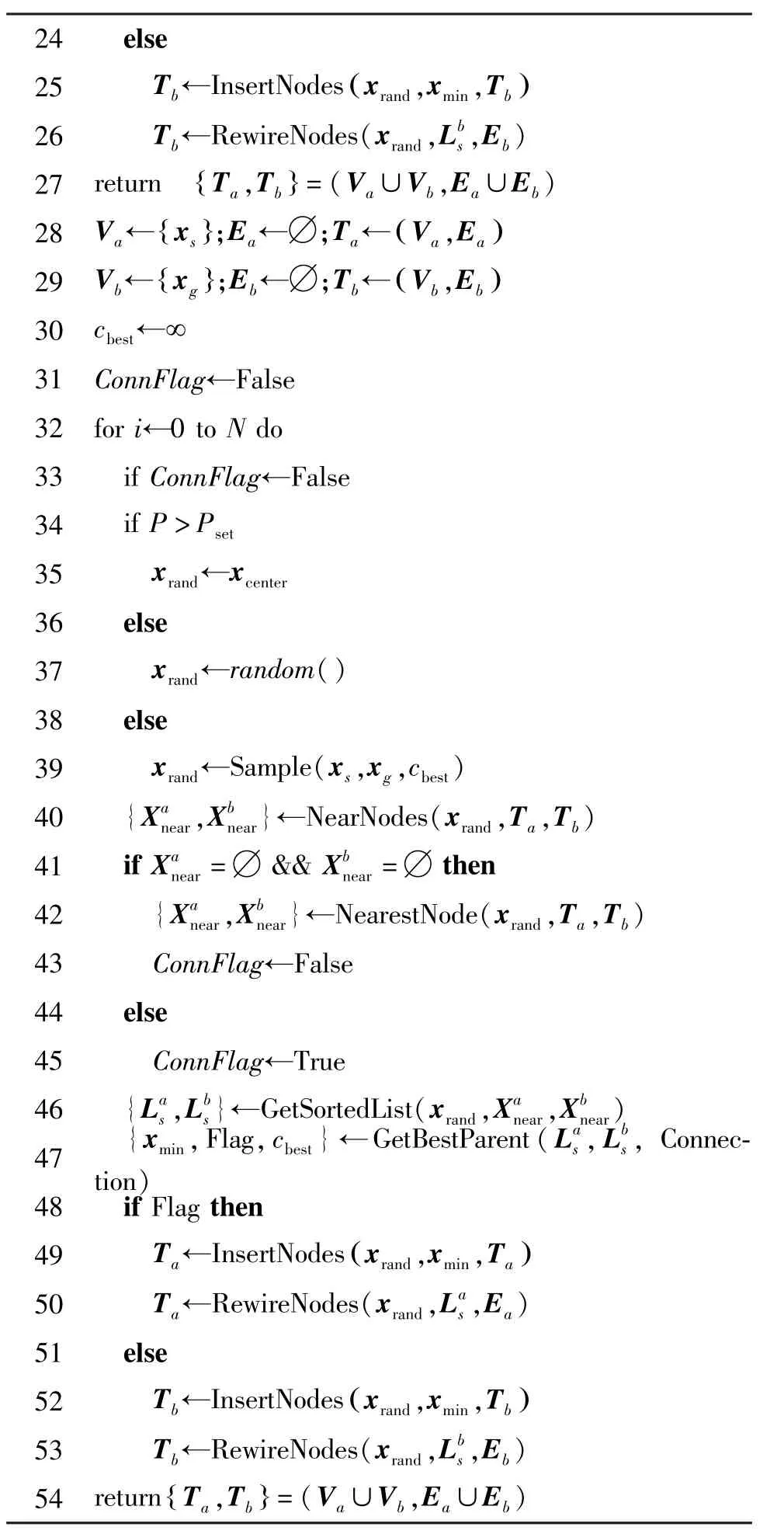
24 else(25 Tb←InsertNodes xrand,xmin,Tb )26 Tb←RewireNodes(xrand,Lb s,Eb){ }=(Va∪Vb,Ea∪Eb)28 Va← {xs };Ea←∅;Ta← Va,Ea 27 return Ta,Tb ( )29 Vb← {xg };Eb←∅;Tb← Vb,Eb ( )30 cbest←∞31 ConnFlag←False 32 for i←0 to N do 33 if ConnFlag←False 34 if P>Pset 35 xrand←xcenter 36 else 37 xrand←random()38 else 39 xrand←Sample(xs,xg,cbest)40 {Xa near,Xb near}←NearNodes(xrand,Ta,Tb)41 if Xa near =∅&& Xb near =∅then 42 {Xa near,Xb near}←NearestNode(xrand,Ta,Tb)43 ConnFlag←False 44 else 45 ConnFlag←True 46 {La s,Lb s}←GetSortedList(xrand,Xa near,Xb near)47 {xmin,Flag,cbest}←GetBestParent(La s,Lb s, Connection)48 if Flag then 49 Ta←InsertNodes xrand,xmin,Ta ()50 Ta←RewireNodes(xrand,La s,Ea)51 else 52 Tb←InsertNodes xrand,xmin,Tb ()53 Tb←RewireNodes(xrand,Lb s,Eb){ }=(Va∪Vb,Ea∪Eb)54 return Ta,Tb

1.4 Probabilistic completeness analysis of the improved IB-RRT∗algorithm

The concept of probabilistic completeness refers to an algorithm's ability to find a path solution with a probability close to 1 when an infinite number of samples are obtained from the configuration space.The IBRRT∗algorithm has been proven to be probabilistically complete in Ref.[16].This paper introduces double elliptical space sampling to address the issue of useless sampling space in the IB-RRT∗algorithm,and the impact on the probabilistic completeness of the algorithm has been proven in Ref.[15].Additionally,the probabilistic central target bias does not restrict the sampling space,ensuring that the improved IB-RRT∗algorithm,incorporating elliptical sampling and probabilistic central circle target bias,remains probabilistically complete.

2 Local path planning based on deep reinforcement learning

The primary challenge in path planning in unstructured environments is the presence of dynamically changing obstacles, such as walking passersby.Although the proposed improved IB-RRT∗algorithm can plan optimal paths based on the relative positions of static obstacles offline,the dynamic random factors will affect the efficiency as well as the safety of the mobile robot.This paper combines the improved IB-RRT∗algorithm to generate the globally optimal path with a deep reinforcement learning algorithm,and trains it on a social attention neural network,to effectively avoid dynamic obstacles.

2.1 Markov decision process model

In this paper,a deep Q-network method is introduced to handle the challenge of dynamic obstacles in path planning.The corresponding Markov decision process MDP(S,A,P,R,γ) can be described by a five-tuple,where the state transfer probabilities isP.The design process ofS,AandRare given as follows.

(2) Action spaceA: the robot can change its speed immediately according to the action command at timet.This section defines the action space during the navigation of the mobile robotA=vtandA∈(0,0.5).

(3) Reward functionR: The designed reward function must be consistent with a purpose,i.e.,avoiding obstacles and keeping a safe distance.During the reinforcement learning training,the intelligence should comply with the following principles.

A larger reward value is given if the robot reaches the target position.

If the interval distance between the robot and the obstacle is greater than 0 or less than a set threshold of 0.3,a penalty value within the range of -0.15 to 0 is given.If the minimum interval between the robot and the obstacle is less than 0,a fixed penalty value is given to the intelligent body.

No reward or punishment is given if other situations arise,such as the robot being far away from an obstacle.

Based on the above discussion,the reward function is designed as follows.

wheredindicates the distance between the robot and the obstacle during the timeΔt.

The optimal value function is defined for the joint stateKtat timetas follows.

whereTis the total number of steps from thetmoment state to the final state,Δtis the time interval between two actions,γ∈(0,1) is the discount factor,vprefis the preferred speed,andR(Kt,at) is the corresponding reward within timet.

The optimal policy is derived from the joint stateaction value function,which maximizes the cumulative reward.

whereP(Kt+Δt,at,Kt) is the transfer probability fromKttoKt+Δtstate when executing the action.

2.2 Value network

The core problem in the Markov decision processlies in determining the optimal value functionV∗(Kt),but the computational complexity of the general iterative algorithm depends on the dimensionality of the joint states.The higher the number of dimensions,the higher the computational complexity.The advantage of deep reinforcement learning is its ability to reduce the computational effort by fitting the optimal value function using neural networks.Therefore,the deep neural network architecture in Ref.[21] was adopted to capture the relative importance of each element of the joint stateKt,which has the advantages of accurate model prediction and a simple structure compared to other neural networks.The value network structure is shown in Fig.4.The input in the figure is the joint state of the robot and the obstacle,and the output is the estimate of the optimal value function.

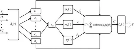
Fig.4 Value network structure

The value network constructed in this section consists of four multilayer perceptron with nonlinear activation functions.First,the multilayer perceptronδe(·)is used to learn the states of the robot and each obstacle and embed weights for each element to produce a fixed-length vector.Second,the embedded vectors are fed into the multilayer perceptronφh(·) to obtain the interactive features of the robot and the obstacles.Again,the embedded vector is fed into another multilayer perceptronρβ(·) to obtain the acquired score for each obstacle.The linearCcombination of the obtained acquired score-weighted interaction features is used as the obstacle features.Finally,the multilayer perceptronζf(·) calculates the values of the obstacle and robot interaction features as estimates of the optimal value functionV∗(Kt).The update rule for each multilayer perceptron is as follows.

According to the above social concern network update rules,the final algorithm is as follows.First,the value network,and experience replay pool are initialized,and the target network is set (Algorithm 3, row 1).The random state is initialized,according toεthe greedy strategy in selecting the action.The reward value and the state of the next moment are got (Algorithm 3,rows 3 to 7).The updated reward value and state are stored in the experience pool and the current value network is updated by gradient descent until the robot exceeds the set maximum time or reaches the final state(Algorithm 3,rows 8 to 11).When the training times reach the set update interval,the target network is updated once (Algorithm 3,rows 12 to 13).The specific value network training pseudo-code is shown in Algorithm 3.

Algorithm 3 Value network training 1 Initialization V,E,V′←V;2 for i=0 to M do;3 Initialization Kt=0;4 repeat 5 at←{RandomAction(),ε argmax at∈A RK(Kt,at)+γΔt·vpref·V∗(Kt+Δt),1-ε;6 R←R(Kt,at) +γΔt·vpref·V′(Kt+Δt);7 status←Kt+Δt;8 Store experience in E 9 Optimizing V with E 10 t←t+Δt,Kt←Kt+Δt;11 until t>tmaxor Kt =Kend;12 if i=M then 13 V′←V;14 end 15 end 16 return V;

2.3 Fusion algorithm

Traditional path planning consists of global path planning and local path planning.The prior knowledge of the environment is used in the global planner to find a best path,and the global plan is adjusted by the local planner to avoid dynamic obstacles.First,a globally optimal path is generated using the improved IBRRT∗algorithm.During the navigation process,if the robot encounters obstacles,a locally optimal path is planned using deep reinforcement learning to avoid the obstacles.Once the obstacles have been avoided,the robot returns to the global optimal path.As depicted in Fig.5,when encountering obstacles,the deep reinforcement learning algorithms determine a new direction.

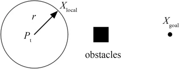
Fig.5 Avoid the obstacles

Based on the above dynamic obstacle avoidance mechanism,the improved IB-RRT∗algorithm for global path planning and the deep reinforcement learning method for local planning are fused by combining global path planner and local path planner to ensure the global optimality of the dynamically planned path.A two-dimensional grid map is established by LiDAR,and a globally optimal and feasible path is planned using the improved IB-RRT∗algorithm.Then a deep reinforcement learning method is used to achieve local dynamic obstacle avoidance,and the optimal strategy is used to select the optimal action so that the robot can quickly find the shortest path to avoid dynamic obstacles in local planning.The algorithmic flow of the fusion algorithm is shown in Fig.6

Fig.6 Flow chart of fusion algorithm

3 Global path planning based on improved IB-RRT∗algorithm

3.1 Simulation

The hardware environment used for the simulation is a computer with Intel(R) Core(TM) i7-9750H CPU@ 2.6GHz and 8GB RAM on Windows 10,and the software environment is Matlab R2018b.To verify the effectiveness of the improved IB-RRT∗algorithm,the Informe-RRT∗,Bi- RRT∗,IB-RRT∗,the improved IBRRT∗algorithms are applied in this section to the twodimensional environment map for global path planning,and the advantageous performance of the improved IBRRT∗relative to various algorithms in terms of finding the initial path speed,algorithm time consuming,and path cost is compared and analyzed respectively.

800 ×800 pixel ratio region with multiple horizontal bars of obstacles is used as the two-dimensional simulation environment, and algorithms comparison results are given in Fig.7, where black pixels are the space occupied by obstacles,white pixels are the free space without obstacles,dotted lines are random search trees,and the upper left corner is the initial position and the lower right corner is the target position.The initial parameters of the algorithm are as follows: initial positionxs= (150,255) ,target positionxs= (650,600),numberN=5000 of iterations,optimal path costcbest=2000,setp=20,and distance thresholddisTh=20,i.e.,the nodes within the distance threshold are considered as the same node.

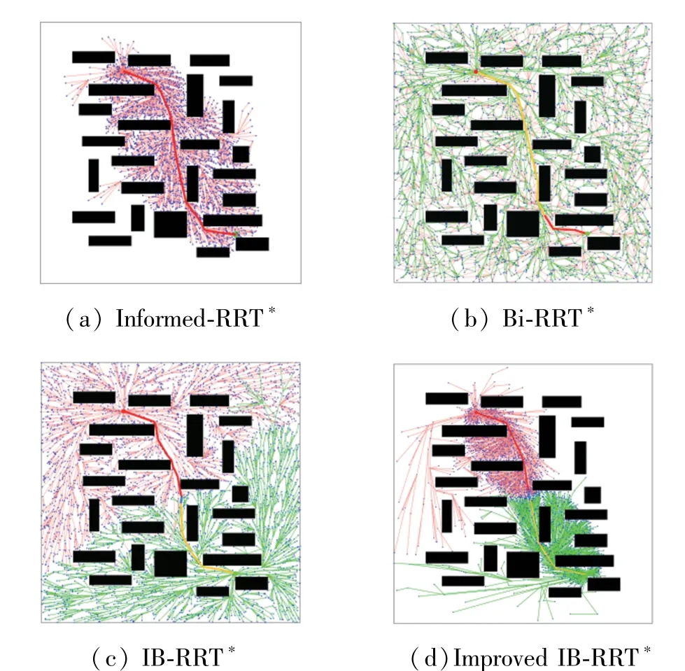
Fig.7 Algorithm comparison chart

Table 4 Algorithm performance comparison

From Table 1 and Fig.8, it can be seen that after 5000 iterations, the optimal path cost of informed-RRT∗is 688.259, smaller than that of Bi-RRT∗and IB-RRT∗, and its corresponding fast random search tree has fewer nodes,but it takes a longer computation time.The initial path can be found faster in the Bi-RRT∗algorithm by setting two subtrees to grow from the initial position and the target position until the two subtrees are interconnected,but the fast random search tree has twice as many nodes as the informed-RRT∗algorithm and the path length is longer.The RRT∗algorithm has more nodes and longer optical path lengths.

The initial path can be found in the improved IBRRT∗algorithm with a minimum number of iterations,which is faster than the other three algorithms.After finding the initial path,the current path is quickly optimized in the initial sample sampled in the elliptic subset sampling domain,and the number of nodes is reduced by 20.14% and the optimal path length is improved by 2.17%.Therefore,compared with the IBRRT∗algorithm,the initial path of the improved IBRRT∗algorithm is faster,the planning efficiency is higher,and the path is higher.

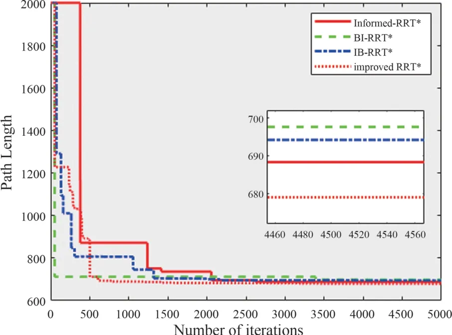
Fig.8 Path length comparison chart

The value network is trained in a simulation environment built with the OpenAI-Gym library.The hidden layerδe(·)sizes inφh(·),ρβ(·) andζf(·)are set to (150,100),(100,50),(100,100),and(150,100,100),respectively.ris set to 0.30m,vprefis set to 1 m/s,andΔtis set to 0.3 s,tmaxis set to 25 s.In this paper,the optimal mutual collision avoidance strategy is used[24]to perform simulated navigation,3000 demonstrations are completed by using the strategy,and then the model is trained every 50 steps by using the gradient descent method with the learning rate set to 0.01 and a discount factor of 0.9.A total of 10 000 training sessions is conducted,where the egreedy strategy decays from 0.5 to 0.1 for the first 4000 sessions and remains constant thereafter.The value network is optimized using 100 training samples and a learning rate of 0.001 for each training.The target value network is updated every 50 steps, and about 18 h are taken during the whole training process,and the robot successfully reached the target with 99% collision-free and 1% collision rate in 500 test cases with the same simulation settings,and the average time to reach the target was 10.68 s.The simulation parameters are shown in Table 2.

Table 2 Simulation training parameters

Fig.9 represents the experimental data.When the training reaches 10 000 times,the cumulative return obtained by the model tends to converge with the convergence value around 0.3174,the collision rate tends to 0,the success rate tends to 99%,and the time to reach the target point is 11.08 or so.It means the model is trained.

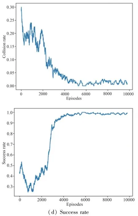
Fig.9 Experimental data

The simulation results of the DRL model for local planning are depicted in Fig.10.The dynamic obstacle,simulated as hollow circls, is controlled by the ORCA algorithm,and the solid circls represent the movement trajectory of the mobile robot.The results show that the mobile robot successfully avoids obstacles and demonstrates a satisfactory avoidance performance.

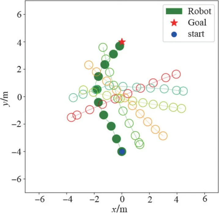
Fig.10 Simulation path diagram

3.2 Real environment experiments

The robot used in the experiment is the Turtlebot 2 mobile robot.The robot is equipped with a computer and Hokuyo LIDAR.The robot's substructure is flanked by differential drive motors,and the movement is controlled by two brushed motors with encoders through the Arduino motherboard,which provides speed control for the robot.

The feasibility of the algorithm was verified using the Turtlebot2 robot in a static obstacle environment and dynamic obstacle environment respectively.2 experimental environments with the same smoothness of the ground, circles on a dotted line in the raster map represent robots,block objects for static obstacles,and circles not on the dotted line represent dynamic obstacles (pedestrians) as shown in Fig.12 and Fig.13.The experimental steps of the specific fusion algorithm are described as follows.

(1) Load the created complete raster map and set the starting position of the mobile robot and the global target point.

(2) Using the robot's AMCL localization method,the real-time robot position information is obtained by odometer calculation,and then the global path from the robot's current position to the global target point is planned by the improved IB-RRT∗algorithm.

(3) Based on the robot's current position information,combined with LIDAR to obtain information on unknown obstacles,DRL local path planning is carried out based on the global path,and the action is selected according to the optimal strategy to return to the global reference path after avoiding dynamic obstacles by using the local dynamic target mechanism.

(4) Determines whether the robot reaches the global target point.The autonomous navigation task is completed if the robot reaches the specified target point.Otherwise,if the target point is not reached,it returns to step (3) to continue the movement.

During the experiment,the experimental parameters of the robot are set as follows: the maximum linear velocityiis 0.5 m/s,the maximum angular velocity is 1 rad/s,the expansion radius of the obstacle is 0.3 m,the robot radius is 0.2 m, the sensor upload information frequency is 5.0 Hz,and the map update frequency is set to 0.5 Hz.

Environment 1 is an arc-shaped corridor as shown in Fig.11,placed with several static obstacles.The actual length of the corridor in Fig.11 is 12.8 m, and its width is 6.8 m.The resolution of the raster map shown in Fig.12 is 20 cm × 20 cm,the starting point is(2.8 m,3.6 m),the target point is set to (2.8 m,10.8 m).The robot ultimately reaches the target point according to the proposed method, as shown in Fig.12,with an error of 0.24 m.

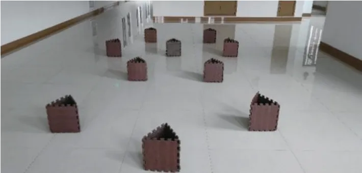
Fig.11 Curved corridor

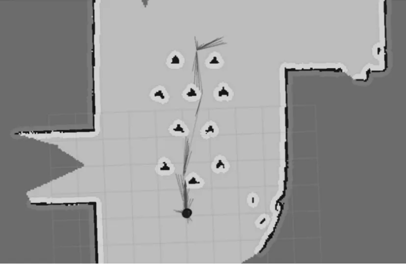
Fig.12 Robot path trajectory

Environment 2 is the same arc corridor as environment 1,and the static obstacles are replaced with dynamic obstacles.Here,this work uses pedestrians as dynamic obstacles,and the movement state of pedestrians is random and can appear from any position within the field of view of the robot,setting the starting point as (1.6 m,0.4 m) and the target point as (1.2 m,0.4 m).Fig.13 (a)shows the pedestrian and robot in the real environment;Fig.13(b) shows that the robot detects a walking passerby in front of it (the circle in the figure represents the pedestrian);Fig.13(c) shows that the robot can predict that the traveler tends to walk to the left (the arrow in the figure);Fig.13(d)shows that the robot returns to the global reference path after bypassing the dynamic obstacle (the solid line is the global reference path,and the dotted line indicates the actual trajectory the robot walked),and finally reaches the specified target point with an error of 0.28 m from the desired target point.

The experimental results demonstrate that the fusion algoritam presented in this paper can perform dynamic obstacle avoidance,and after bypassing pedestrians,it can quickly return to the global reference path,basically follow the planned path to reach the designated target point,and ensure that the planned path has global optimality.Due to the inaccurate map positioning, deviation of odometer calculation, and the possibility of sliding between the robot and the ground,there is an error between the robot’s actual arrival at the target point and the expected target point, but the error does not exceed 0.30 m,which is sufficient for the practical needs and applications.

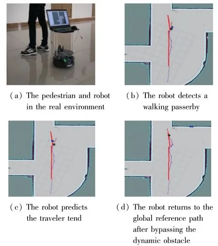
Fig.13 Local dynamic obstacle avoidance effect

4 Conclusion

This paper proposes a dynamic fusion path planning algorithm for mobile robots that integrates an improved IB-RRT∗algorithm with deep reinforcement learning for real-time global and local path optimization.The improved IB-RRT∗algorithm addresses the issues of excessive search nodes and long planning path length present in the traditional IB-RRT∗approach.Simulation results demonstrate that the improved IBRRT∗algorithm outperforms the traditional Bi-RRT∗,Informed-RRT∗,and IB-RRT∗algorithms in terms of path length and number of search nodes.To overcome the limitations of the traditional local planning algorithm in dealing with dynamic obstacles,a deep reinforcement learning approach is introduced for local path planning.The experiment shows that the fusion algorithm can effectively avoid dynamic obstacles,predict the movement trend of dynamic obstacles,and improve the efficiency and safety of autonomous robot navigation,verifying the effectiveness of the proposed fusion algorithm.