Prediction of permeability from well logs using a new hybrid machine learning algorithm
2023-08-30MortezMtinkiRominHshmiMohmmMehrMohmmRezHjseeiArinVelyti
Mortez Mtinki ,Romin Hshmi ,Mohmm Mehr ,Mohmm Rez Hjseei ,Arin Velyti
a Department of Petroleum Engineering,Omidiyeh Branch,Islamic Azad University,Omidiyeh,Iran
b Department of Applied Mathematics,Faculty of Mathematics and Computer Sciences,Amirkabir University of Technology,Tehran,Iran
c Faculty of Mining,Petroleum and Geophysics Engineering,Shahrood University of Technology,Shahrood,Iran
d Department of Chemical and Materials Engineering,University of Alberta,Edmonton,Canada
Keywords:Permeability Artificial neural network Multilayer perceptron Social ski driver algorithm
ABSTRACT Permeability is a measure of fluid transmissibility in the rock and is a crucial concept in the evaluation of formations and the production of hydrocarbon from the reservoirs.Various techniques such as intelligent methods have been introduced to estimate the permeability from other petrophysical features.The efficiency and convergence issues associated with artificial neural networks have motivated researchers to use hybrid techniques for the optimization of the networks,where the artificial neural network is combined with heuristic algorithms.This research combines social ski-driver (SSD) algorithm with the multilayer perception (MLP) neural network and presents a new hybrid algorithm to predict the value of rock permeability.The performance of this novel technique is compared with two previously used hybrid methods (genetic algorithm-MLP and particle swarm optimization-MLP) to examine the effectiveness of these hybrid methods in predicting the permeability of the rock.The results indicate that the hybrid models can predict rock permeability with excellent accuracy.MLP-SSD method yields the highest coefficient of determination (0.9928) among all other methods in predicting the permeability values of the test data set,followed by MLP-PSO and MLP-GA,respectively.However,the MLP-GA converged faster than the other two methods and is computationally less expensive.
1.Introduction
Accurate estimation of the petrophysical properties such as permeability,porosity,water saturation,density,and lithology is of utmost importance in the evaluation of the hydrocarbon reservoirs.Such characterization is primarily based on the measurements obtained by well logs,core sample testing,well testing,field production data,and seismic information [1].Various empirical correlations have been presented for the estimation of petrophysical data from the well log measurements.However,these correlations are often limited to a single well only and may not apply to other wells even if the geological features of the wells are relatively similar [2].Hence,the problem with the correlations developed using regression techniques appears to be the non-uniqueness of the equations which arises from introducing insufficient parameters into the models.
Permeability is a petrophysical property of the rock that represents the displacement of the fluids in the porous media.This is an essential parameter for reservoir evaluation,management,and selecting the optimum enhanced oil recovery method.Permeability is generally measured either by coring from the formations or downhole pressure testing methods.The coring test results are“local” and belong to a minute section of the reservoir.Downhole pressure tests account for the anisotropic nature of the formation but yield in a single value.These techniques are costly and timeconsuming [3].
Extrapolating values from insufficient permeability measurements can be erroneous due to the high uncertainty associated with the “local” nature of these techniques.Moreover,such measurements are not always available.Therefore,researchers have attempted to correlate the permeability to the other petrophysical properties obtained from the well logs [4].Measurements from coring are always used for calibrating the predicted results.
Kozeny [5] and Carman [6] developed the first correlation (KC correlation)of this type,in which permeability is correlated to the formation porosity.Later on,modifications to the KC correlation were presented by other researchers [7,8].The application of such equations is essentially limited to unconsolidated homogeneous sands due to the assumptions used in developing the analytical correlations.
Most of the presented equations have limited application due to the existing heterogeneity of the reservoirs.The findings clarify that permeability cannot be simply correlated to the porosity only and many other factors involved must be incorporated into the correlation.Such includes more petrophysical parameters such as radioactive,electrical,and sonic properties which can resolve the non-uniqueness problem of such correlations.
Advanced methods and intelligent techniques have been proposed to address the issue of the non-uniqueness of the presented correlations.For instance,Multivariate Regression Analysis (MRA) method was applied to address the models' generalization problem [9].Moreover,Artificial Neural Networks (ANN) method has been used and gained popularity recently as an alternative to the MRA and the results obtained from the utilization of this intelligent method have been reported to be positive[10,11].Other approaches such as fractals and multifractal theory,statistical approaches,and methods based on percolation theory have been used extensively and successfully in the estimation of the petrophysical properties [3].Furthermore,intelligent methods can be employed to deal with the problem of the spatial distribution of the properties in the formation[12].
Hybrid artificial intelligence-optimization algorithms have been utilized for the prediction of reservoir petrophysical properties.Evolutionary optimization methods are often used to achieve the optimum network structure and improve the convergence and efficiency of the network.Many studies of this type are available in the literature,where the petrophysical properties of formations are estimated from the well logs [13-16].
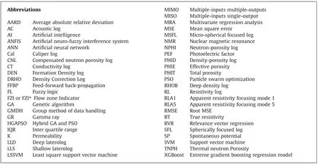
Mulashani et al.[17] applied enhanced group method of data handling(GMDH)which uses modified Levenberg-Marquardt(LM)to predict permeability from well logs.Otchere et al.[18] used extreme gradient boosting(XGBoost)regression model to estimate reservoir permeability and water saturation.Zhang et al.[19]combined petrophysical rock typing method(FZI or FZI*)with PSOSVM algorithm to predict permeability and porosity from GR,DEN,and DT.Nkurlu et al.[20]estimated permeability from well logs by using GMDH neural network.Okon et al.[21] developed a feedforward back-propagation (FFBP) artificial neural network (ANN)model with multiple input multiple out (MIMO) structure.Adeniran et al.(2019) introduced a novel competitive ensemble machine learning model for permeability prediction in heterogeneous reservoirs.Ahmadi and Ebadi[22]used the optimized least square support vector machine (LSSVM) and fuzzy logic (FL) to estimate the Porosity and Permeability of petroleum reservoir.Ali and Chawathe[23],studied the relationship between petrographic data collected during thin section analysis with permeability using the artificial neural network (ANN).Chen and Lin [24] used an ensemble-based committed machine with empirical formulas(CMEF)to estimate permeability.Gholami et al.[25]used relevance vector regression (RVR) along with genetic algorithm (GA) as an optimizer to predict permeability from well logs.Jamialahmadi and Javadpour [26] utilized RBF to identify the relationship between porosity and permeability.Verma et al.[27],studied five well log Alberta Deep Basin and used ANN to predict porosity and permeability.Handhel [28] predicted the Horizontal and vertical permeability by backpropagation algorithm from 5 different well logs.Elkatatny et al.[29] developed an ANN with three well logs to predict permeability in heterogeneous reservoirs.In Table 1,the previously used machine algorithms and input parameters for the prediction of permeability are presented.
In this paper,a hybrid MLP-SSD algorithm was designed and employed to estimate the permeability of the formations from the well logs.Social Ski-driver (SSD) is categorized as an evolutionary optimization algorithm (EA) that improves the classification performance,resolving the challenge of imbalanced data associated with robust classification modeling.This algorithm was recently introduced by Tharwat and Gabel [31] and is inspired by different evolutionary algorithms such as PSO,sine cosine algorithm (SCA),and gray wolf optimization (GWO),and its stochastic nature resembles alpine skiing paths.The hybridization of MLP and SSD improves the efficiency of the computations.As shown in Table 1,the proposed hybrid algorithm has not been used previously to predict the permeability of the rock.The performance of this hybrid model was compared to MLP-PSO,MLP-GA,and MLP models,and it was found that the MLP-SSD algorithm is superior in terms of model accuracy.
In section 2,the methodology and workflow of the research are described.In section 3,the type and statistics of the collected data are presented and section 4 contains the results and discussions on the quality of input data,algorithm training,and the performance of algorithms with the unseen data sets.The conclusions of the study and the description of the advantages and limitations of the introduced model are given in section 5.
2.Methodology
Sampling from wells to perform tests related to determining rock permeability is very time-consuming and costly.Besides,sampling along the entire length of the well for permeability testing is not possible;Therefore,the output of these studies will be discontinuous rock permeability data.Using this method for carbonate reservoirs that have high heterogeneity will not yield acceptable results.Thus,using other tools such as formation microimager (FMI) or formation micro scanner (FMS) to estimate the permeability of carbonate reservoirs,in addition to reducing time and cost,will provide continuous data.The use of permeability test results on core samples is vital to calibrate the values of the FMI/FMS permeability index in this method;to achieve highly accurate and reliable results.
Fig.1 shows the workflow used in this study to extract the permeability index from the FMI graph and its calibration with the results of the permeability test,as well as modeling the permeability using conventional petrophysical graphs.No core sample was taken from the target depth (Fahlian Formation) and the permeability (KFMI) of the FMI output should be corrected for changes in water saturation (Sw).Equation (1) was used for this purpose and the constant(n)in the correlation was determined for Fahlian Formation using FMI graphs and permeability laboratory tests on samples from two other neighboring wells.

Fig.1.The workflow for permeability modeling of the target well.The blue box on the right is a process performed to determine the constant in Equation(1)using the permeability data of the core and the FMI log in two wells from the study field in the Fahlian Formation.The red box on the left represents the process used to determine permeability and model it in the well under study.The data used in this study (ie,conventional good wells and permeability graphs normalized using Equation (1)) are marked in blue.
To model permeability in this study,data preprocessing is first performed to detect and remove outlier data,and select more features that influence permeability.The Tukey method,which is a statistical method based on box plot diagrams of data,was used to detect and remove outlier data [32].Moreover,feature selection was performed by applying the neighborhood component analysis(NCA)algorithm to the database without outliers.In the next step,the selected features were considered as input to the MLP-GA,MLPPSO,and MLP-SSD hybrid algorithms.After training the hybrid models with 80% of the selected data,the trained models were tested with the rest of the data.
2.1.Pre-processing
Data processing is essential for the correct extraction of the governing relationships between inputs and outputs.Applying data preprocessing results in a model with high accuracy and generalizability.Identifying and deleting outlier data and feature selection are two processes that were performed on raw data in this study in the preprocessing stage.
2.1.1.Outlier detection and elimination
Actual data is affected by numerous factors,among which noise is a key factor,leading to inaccurate extraction of the rules governing the data and thus results in the low generalizability of estimator or class models.Exposure to noisy data can be classified into two categories: identifying and deleting remote data andreducing the effect of noise.Since the outlier data have unusual values compared to other observations (i.e.they deviate from other observations),they can be identified by both univariate and multivariate methods.In the univariate method,the data distribution of one property is examined alone,while in the multivariate method,several properties in multidimensional space must be examined to identify remote data.In the noise reduction method,a filter is used to reduce the effect of noise in the data,the intensity of which is proportional to the signal-to-noise ratio in the data.In this method,unlike the first method,the number of data is not reduced,but its values are changed according to the noise intensity.
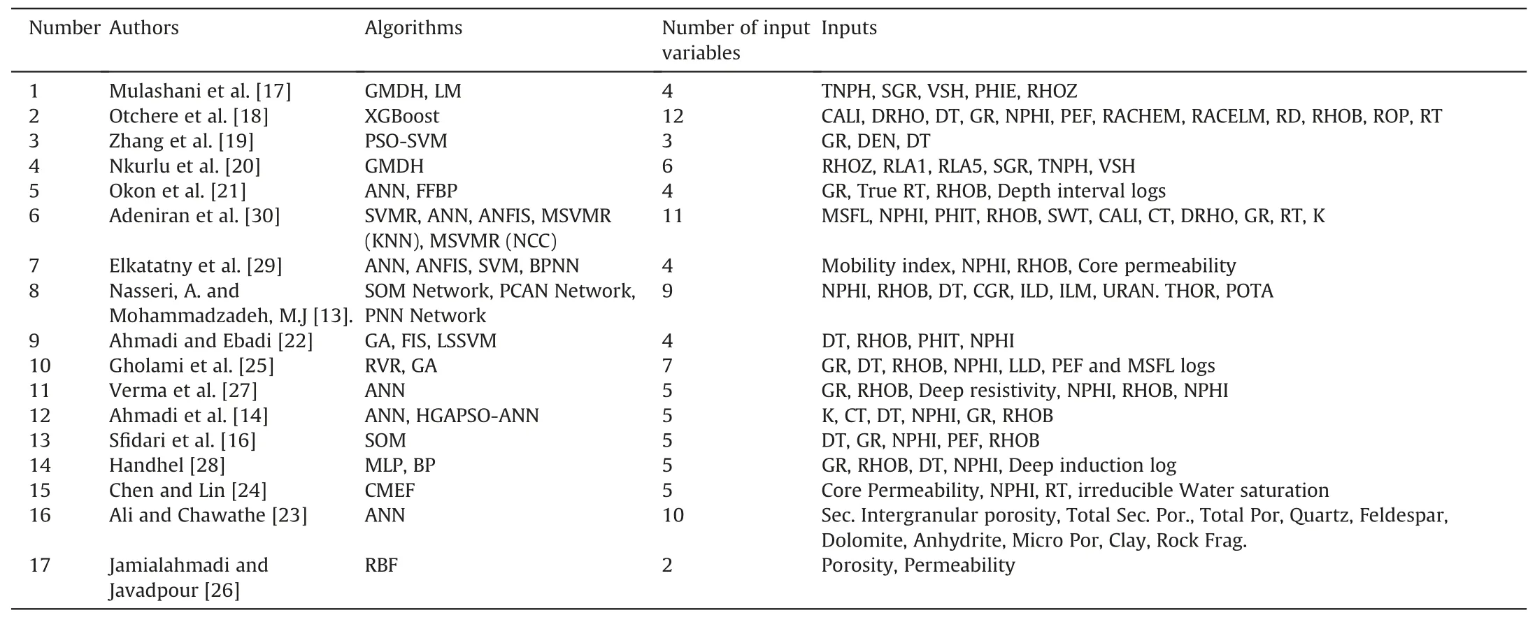
Table 1 Application of machine learning algorithms in the literature review of permeability prediction.
Due to the uncertainty of the signal-to-noise ratio in the data received for this study,the Tukey method will be used to identify and delete outlier data.In this method,by calculating the values of the first quarter (Q1) and third (Q3) for each feature,the interquartile range(IQR)is determined using equation(2).The values of the lower inner fence (LIF) and upper inner fence (UIF) are then calculated separately for each property(Equation(3)and(4)).Data with values less than LIF and more than UIF are identified as outlier data and must be removed from each attribute.
2.1.2.Feature selection
Feature selection is one of the fundamental concepts in data mining that affects the model performance significantly.Therefore,it is important to consider feature selection as the initial step to design the model of interest.Feature selection is a process in which the features with the highest influence on the prediction variable or the desired output are recognized and selected either manually or automatically.Hence,this process reduces a large dimension feature vector into a smaller one by eliminating the irrelevant features.
The inclusion of irrelevant features in the model input data reduces the accuracy and results in the generation of a model based on these features which may affect the application of such poorly developed models.The criterion for feature selection is the numerical value of the feature weight that is evaluated by the feature selection algorithm.At first,the feature selection algorithm should calculate the weight of each feature,and then,the weight of all features is compared with a threshold value.Finally,features with weights higher than the threshold value are selected for the modeling,and the rest are discarded.
Various techniques have been proposed for feature selection which can be categorized into two “Filter” and “Wrapper” groups.In Filter methods,features are designated without training and based on their direct correlation with the output parameter.On the other hand,Wrapper approach employs a series of training processes.Studies favor the Wrapper technique with superior responses compared to the Filter methods [33].This study employs neighborhood component analysis which falls under the Wrapper methods,for feature selection.
Goldberger et al.[34]introduced the neighborhood component analysis as a non-parametric method,aiming to maximize the accuracy of the clustering algorithms and regression.IfS={(xi,yi),i=1,2,…,N} is considered as the training input data,xi∊Rpis a feature vector andyi∊Ris the corresponding output vector.The objective here is to find values for the weight vectorwin 1×pdimension.These values indicate the significance of the features in estimating the response variable.In this method,xjis a sample reference point among all the samples forxisample.Pij;the probability of thexjselection as thexireference point from all the samples is very sensitive to the distance of the two samples.This distance is represented by the weighted distancedw,and is defined via equation (5) [34]:
wherewmis the allocated weight for the mth feature.The correlation between the probabilityPijand the weighted distancedwis made possible by the kornel functionkin equation (6).
Moreover,ifi=j,thenpii=0.Kornel function in equation(7)is defined as follows:
where σ is the kornel width which influences the probability ofxjselection as the reference point.Assumingis the predicted response values by the random regression model for the pointxiandl:R2→Ris the loss function (determines the difference between theyiand),average valueis computed using equation (8):
Leave-one-out is a strategy implemented to increase the accuracy of the regression model.The inclusion of this strategy on the training data S ensures the success of the neighborhood component regression.Summation of training datalidivided by the number of data present in the training data collection is the average accuracy of the leave-one-out regression.Although,this objective function is prone to overfitting.A regularization term λ was introduced to prevent the overfitting of the neighbor component analysis model which has equal value for all the weights in one problem.Therefore,the objective function can be presented as shown in equation (9):
The defined objective in this correlation is known as the regularized NCA.Weight values for the features are introduced to minimize the objective function.Different loss functions such as root mean square error and average absolute deviation may be utilized in equation (9).
2.2.Multi-layer perceptron neural network (MLP-NN)
Artificial neural network (ANN) is one of the data-based modeling techniques that is used extensively to solve complicated problems such as clustering and classification,pattern recognition,and estimation,and prediction.ANN is made of several calculation blocks,known as the artificial neuron,and has a flexible structure that enables the network to model non-linear problems[35].
Multi-layer perceptron(MLP)has been employed repetitively to solve the function estimation problems from the existing types of ANN.This type of network consists of three layers: input,hidden,and output layers[36].The neurons at each layer are connected to the neurons at the next layer using weights with values in a range of [-1,1].Each neuron in MLP-NN performs two summation and multiplication operations on the inputs,weights,and biases[12,36-38].Initially,inputs,weights,and biases are summed up using equation (6):
In this equation n is the number of inputs,Iiis the ith input variable,βjis the bias for the jth neuron andwijis the connecting weight between ith input and jth neuron.
In the next step,an activation function must be applied to the output of the correlation 6.Different activation functions may be utilized in an MLP-NN,of which the most common types are listed in Table 2:
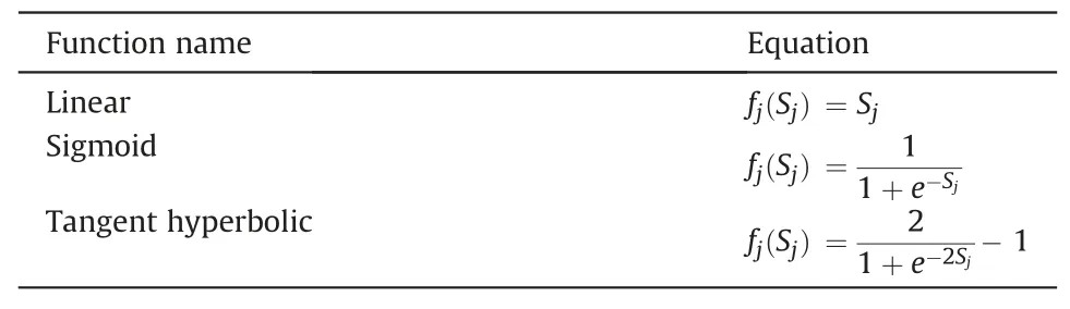
Table 2 Popular activation functions in MLP-NN.
After setting the number of hidden layers and the number of neurons in each layer,the network has to be trained to adjust and update the weights and biases using training algorithms.For this purpose,classic training algorithms are generally applied such as Levenberg-Marquardt (LM),conjugate gradient (CG),Newton method(NM),gradient descent(GD),and quasi-Newton(QN).The selection of the training algorithm must be based on the type of problem that is going to be solved.Nevertheless,LM has been reported to have superior computational speed among all other methods but requires large memory[39].GD algorithm,unlike LM,has lower computational speeds but requires less memory [39].Therefore,in problems with a large amount of data it is better to use GD algorithm to save the memory.
2.3.Optimization algorithms
A review of studies about MultiLayer Perceptron by using different learning Algorithms in the oil and gas industry shows that models that use meta-heuristic optimization algorithms are more accurate and generalizable in comparison with classic algorithms[3].Thus,in this research Genetic,PSO,and Social ski-driver optimization algorithms were used as Neural Network learning algorithms.
2.3.1.Social ski-driver (SSD)
A novel optimization SSD algorithm was introduced in 2019 by Tharwat and Grabel [31].This algorithm is based on a random search,which is somehow reminiscent of a ski rider moving down a mountain slope.The parameters of this algorithm are as follows:
(1) Ski-driver place(Xi∊Rn):This parameter is used to evaluate the objective function in the desired location.The value of n indicates the size of the search space.
(2) Best previous location(Pi):The compatibility value for all ski drivers is calculated with the help of the compatibility function.The calculated value for each factor is compared to the current values and the best one is stored.This value is similar to the particle swarm optimization (PSO)algorithm.
(3) The average of the general Solution (Mi): In this algorithm,like the gray wolf optimization algorithm,the ski drivers pass through the global points and show the best values which are depicted in Fig.2.
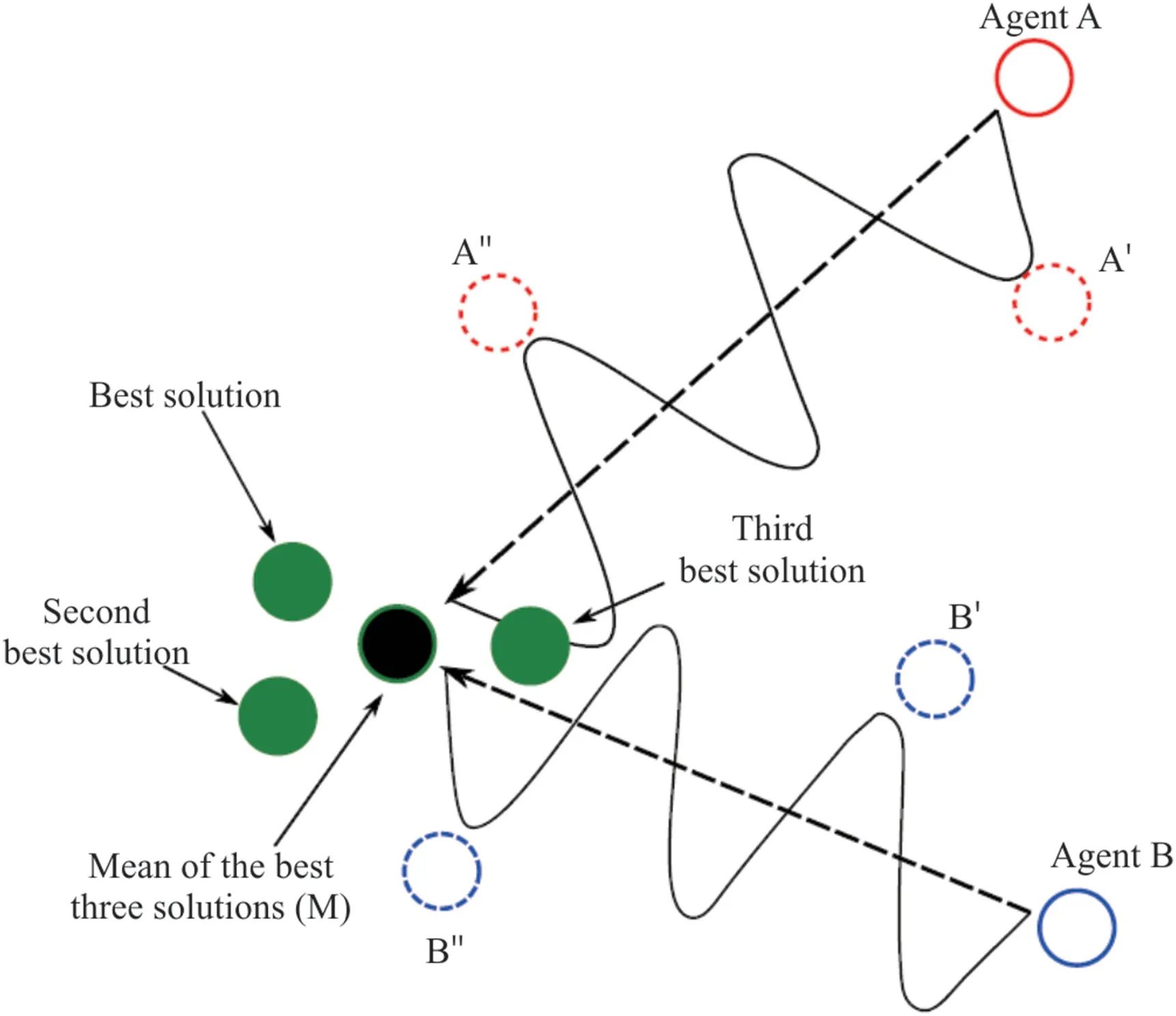
Fig.2.Demonstrate how particles A and B move toward the average of the three best answers using the SSD algorithm.Particle A moves nonlinearly to A′ and then to A′′,as does particle B [31].
whereXα,Xβ,Xγshow the best results in the t-th iteration.
The speed of the ski-driver(Vi):The location of the ski driver is updated by adding speed,and this value is calculated using the following equations:
whereViis velocity ofXiandr1,r2are random numbers that are uniformly generated in the range of 0 and 1.Piis the best solution for the i-th ski-driver,Miis the average of the total solution for the whole population and c is a parameter that is used to create a balance between exploration and extraction,the value is calculated by Equation (14),in which α has a value between zero and one.Increasing the number of repetitions reduces the value of c.Thus,by increasing the number of iterations,the exploratory property of the algorithm decreases,and its focus on the solutions increases.
The main purpose of the SSD algorithm is to search spaces to find the optimal or near-optimal answer.The number of parameters that should be optimized determines the dimension of the search space.In this algorithm,the position of the particles is first randomly set and then the position of the particles is updated by adding speed to the previous position according to Equation (12).Also,the velocity of the particles is created according to Equation(13) as a function of the current position of the particle,the best personal position,and the best position of all particles so far,and based on those particles,move nonlinearly towards the best answer-which is the result of the average of the three best answers that exist right now.This nonlinear motion increases the ability to explore new solutions in the SSD algorithm [31].
2.3.2.Particle swarm optimization
The PSO algorithm was developed by Kennedy and Eberhart[40],inspired by the social behavior of organisms in groups such as birds and fish.Instead of focusing on a single individual implementation,this algorithm focuses on one particle of individuals.Also,in this algorithm,the information of the best position of all particles is shared.Although the convergence rate in this algorithm is high,it is very difficult to get rid of the local optimization if the PSO gets stuck in it [41].
The flowchart of the PSO algorithm is shown in Fig.3.The PSO algorithm finds the best solution in the search space using a particle population called congestion.The algorithm starts by initializing the population position randomly in the search space (lower and upper limit of decision variables) and initializing the speed between the lower limit (Vmin) and the upper limit ((Vmax).The specified locations for the particles are stored as their best personal position (Pb).The position of all particles is evaluated by the objective function,and the particle with the minimum value of the objective function is selected as the best global position (Gb).In each iteration,the new velocity (Vi(t+1)) for each particle (i) is defined based on the previous velocity (Vi(t)) and the distance of the current location (xi(t)) from the best personal and global positions,which is shown in equation (15) [42].Subsequently,the new situation of the particle (xi(t+1)) is calculated based on the previous position and the new velocity (Equation (16)).The new location of the particles is then assessed with the objective function.iterations continue until the termination conditions are reached.This algorithm is a very suitable method for continuous problems due to its continuous nature.

Fig.3.PSO algorithm flowchart [11,46-48].
wherei=1,2,…,n,andnis the number of particles in the swarm;w is Inertial weight (the amount of recurrence that controls the particle velocity) [43,44] and the range [0.5,0.9] improves the performance of the PSO algorithm(Martinez and Cao,2018));c1,c2which are positive coefficients,are called personal and collective learning factors,respectively,andr1,r2are random numbers in the range[0,1] [44,45].
2.3.3.Genetic algorithm
Genetic algorithm is a type of evolutionary algorithm which was introduced by Holland and is inspired by the science of biology and concepts such as inheritance,mutation,selection,and combination[49,50].Fig.4 shows how the genetic algorithm works to find the optimal solution.As shown in this figure,a genetic algorithm,like other evolutionary algorithms,begins with an initial population of randomly generated chromosomes.Each of these chromosomes is then evaluated with an objective function that allocates a value called fitness to them.In the next step,chromosomes participate in the reproduction process (crossover operation) as parent chromosomes according to the amount of fitness function they have.The lower the cost function,the more chances chromosomes have for reproduction.Next,the mutation operation is used to produce the population of the next generation of chromosomes.Due to its random nature,this operation allows escaping from local optimal points.However,if elitism is used,it can be guaranteed that by doing this process,the next population will be at least as good as the current population.Crossover and mutation operations in the genetic algorithm regulate its exploitation and exploration properties,respectively.The whole process is repeated for future generations and continues until the algorithm terminates [51].

Fig.4.GA optimization flowchart [52,53].
2.4.Developing hybrid algorithms
After determining the structure of the multilayer perceptron neural network,adjusting the values of weights and biases is of particular importance and strongly affects the accuracy of the developed model.Due to the better performance of meta-heuristic algorithms in neural network training and determining the optimal values of weights and biases compared to classical optimization algorithms,GA,PSO and SSD will be used as neural network learning algorithms.
Fig.5 shows the hybrid steps of the MLP-GA,MLP-PSO,and MLPSSD algorithms.After separating the data into two categories of training and testing,the neural network designed is trained with the LM optimization algorithm.Weights and bias values are then extracted in the trained model and considered as the best current values of all factors (particles or chromosomes) in meta-heuristic optimization algorithms.Also,the sum of the number of weights and biases is defined as the number of decision variables (search space)in these algorithms.Fig.6 shows how to extract the values of weights and biases as well as their number for the MLP-NN Algorithm with one hidden layer.The optimization algorithms used,with a certain number of iterations and a specific population,are implemented to determine the optimal values of the decision variables (i.e.weights and biases) to minimize the model estimation error.After stopping the optimization operation based on the specified conditions,the obtained optimal values of weights and biases are placed in the MLP model.Finally,the MLP-GA,MLP-PSO,and MLP-SSD hybrid models are evaluated with test data.
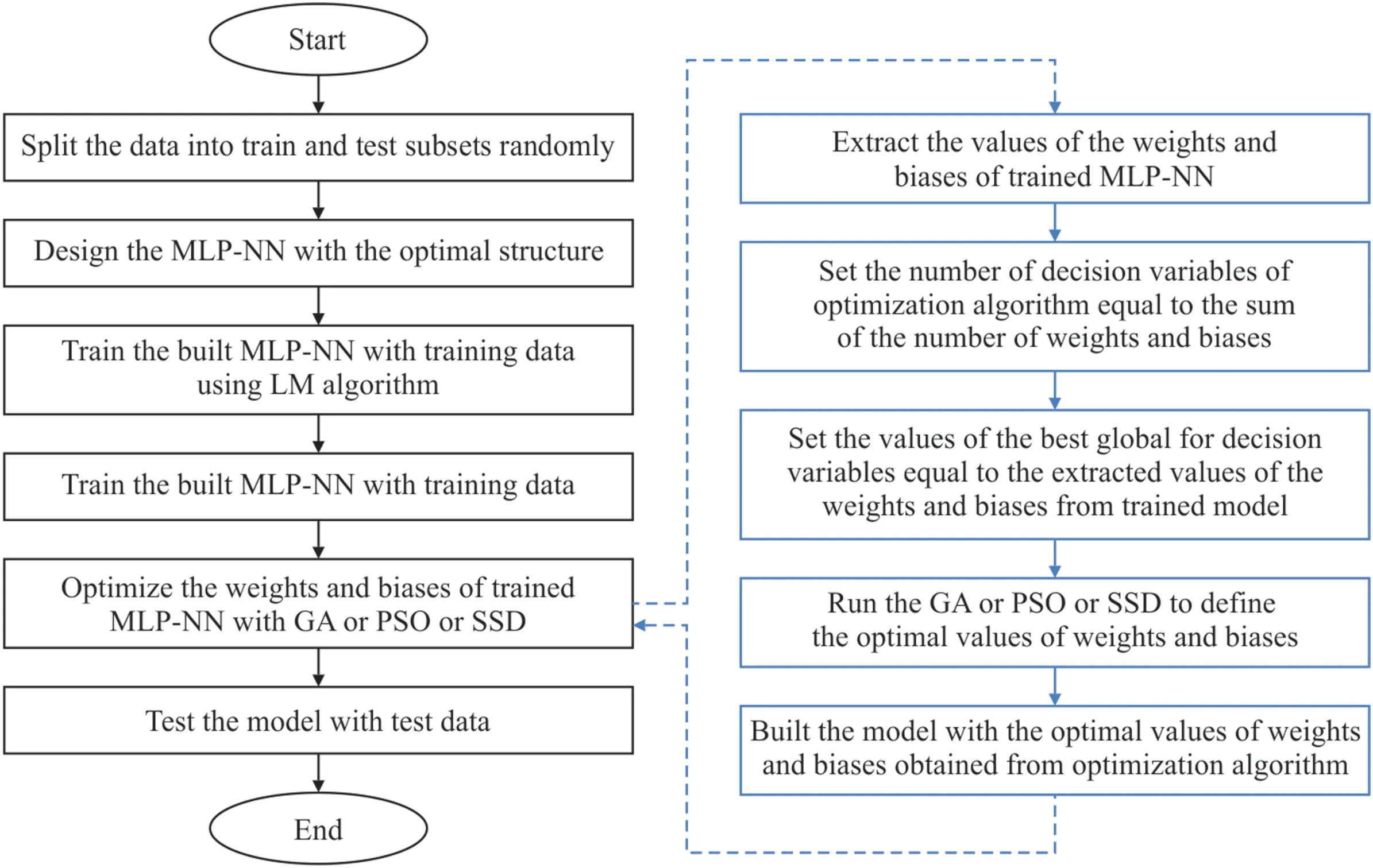
Fig.5.MLP-GA,MLP-PSO and MLP-SSD hybrid algorithm development flowchart.
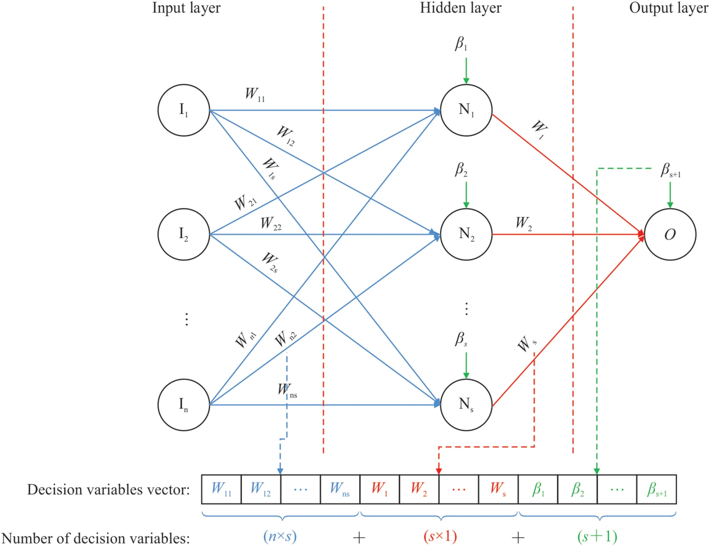
Fig.6.Extracting weights and biases in the form of decision variables vectors and the number of these variables for a hidden single-layer MLP-NN in order to optimize their values with meta-heuristic algorithms.
3.Gathered data
The data collected in this study include petrophysical logs(depth,calorimetry,corrected gamma,photoelectric coefficient,neutron porosity,density,true resistance,and time of compression wave travel)and corrected permeability for the area of the Fahlian Chahi Formation in one of the southwestern field of Iran.Due to the high heterogeneity in this carbonate formation,which consists of limestone,the use of FMI can provide a good permeability profile.Table 3 shows the range of variations of each feature along with some statistical indicators for the collected data.Fig.7 shows the log of changes in the values of each feature in the Fahlian Formation of the studied well.According to this figure the increase in the diameter of the well,especially in the approximate range of 4400-4420 m,has affected the values of the harvested characteristics.Therefore,preprocessing seems necessary to remove outlier data.
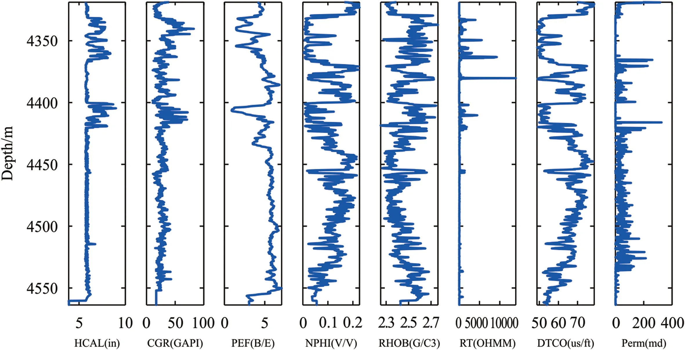
Fig.7.Profile of depth changes of the values for each parameter in the Fahlian Formation of the studied well.
4.Results and discussion
Based on the initial evaluations,the values of the harvested logs are affected by noise.Therefore,the Tukey method was used to remove the outliers.IQR was calculated using the values of the first and the third quartiles.and the upper and lower limits were determined.Accordingly,339 data points (i.e.,21% of data) were identified as outliers and were removed.
Fig.8 shows the matrix of Pearson correlation coefficients between the features.There is no significant relationship between the corrected gamma and permeability in the studied well.In contrast,the porosity,density,and compressional travel time of sonic waves have the highest correlation with permeability.Porosity and compression wave travel time are directly related,and density is inversely related to permeability.
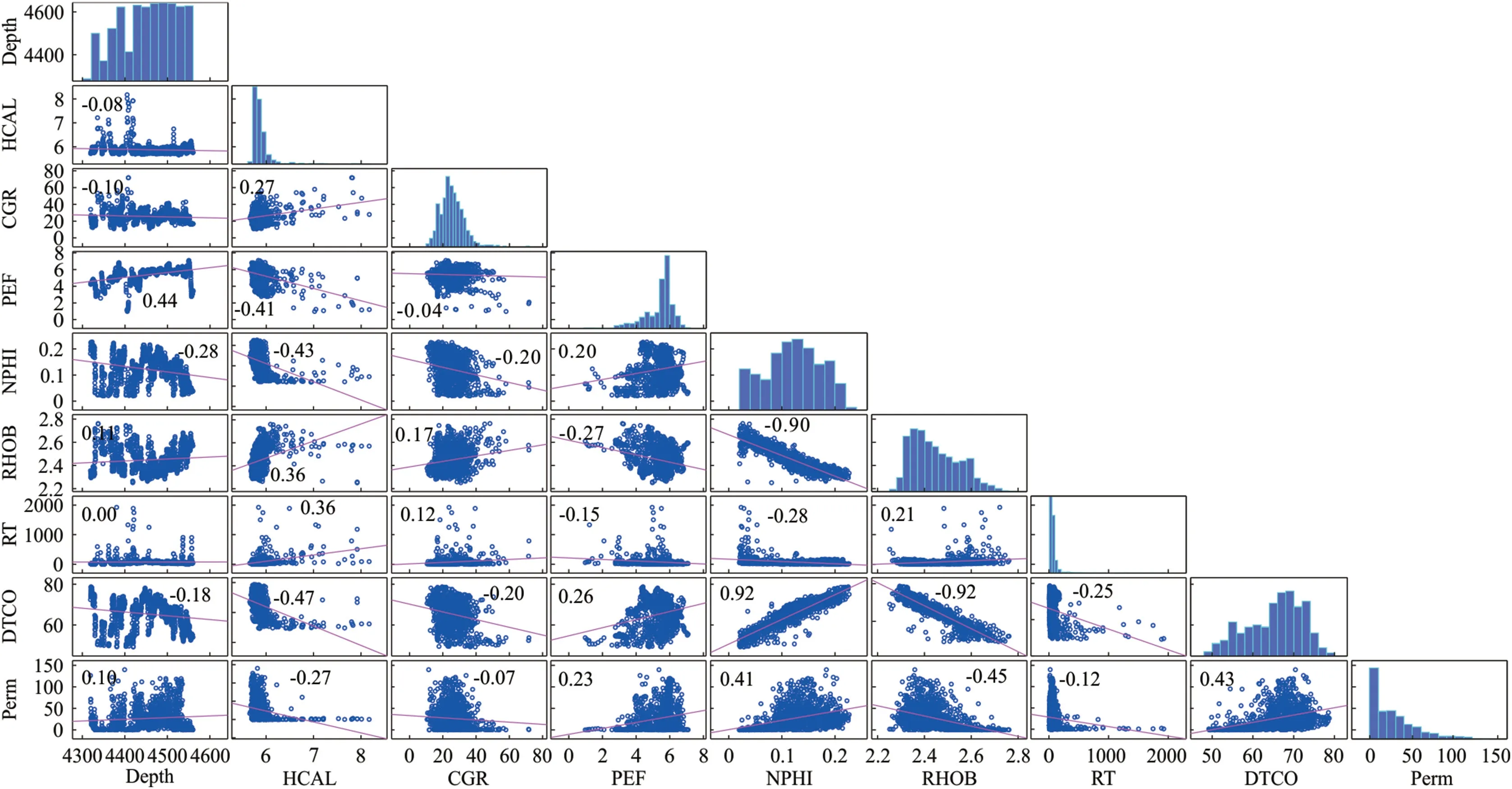
Fig.8.Matrix diagram of pairwise comparisons of independent and dependent parameters in the studied well after removal of outliers.
It is necessary to apply the NCA algorithm to the data for the feature selection among the given variables.However,the data first needs to be normalized and then the optimal lambda value in Equation (9) must be calculated.For mapping data between 1-and +1 by specifying the maximum values (Xmax) and minimum(Xmin) for each attribute,the mapped values (Xnorm) can be determined using Equation(17).To ascertain the optimal lambda value,the amounts between zero and 1.3 were defined with a step of one hundred-thousandth,and then with the k-fold cross-validation algorithm,the RMSE quantity for each of the lambda values was determined to estimate the permeability based on all inputs.The sensitivity analysis implies the number of folds in the k-fold crossvalidation algorithm for this problem was considered 10.Fig.9 shows the error value for different lambda values for estimating permeability using all inputs.As can be seen in this figure,the best value for lambda to achieve the lowest error in the estimate is 0.13669.Therefore,this value was defined in Equation(9)to specify the properties with the greatest effect on permeability for lambda.

Fig.9.RMSE changes for different lambda options in the NCA feature selection algorithm.
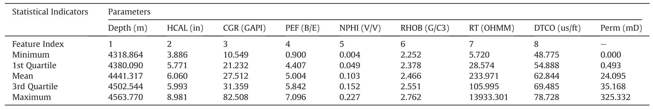
Table 3 Range of changes of each feature along with some statistical indicators for the data recorded in Fahlian Formation of the studied well.
Fig.10 shows the values obtained for each of the features in the permeability estimation using the NCA algorithm.As can be seen in this figure,the properties of depth,porosity,true resistance,and compression wave travel time have the highest value (effect) in permeability estimation.Therefore,these properties were considered as the input of hybrid models for permeability estimation in the modeling stage.
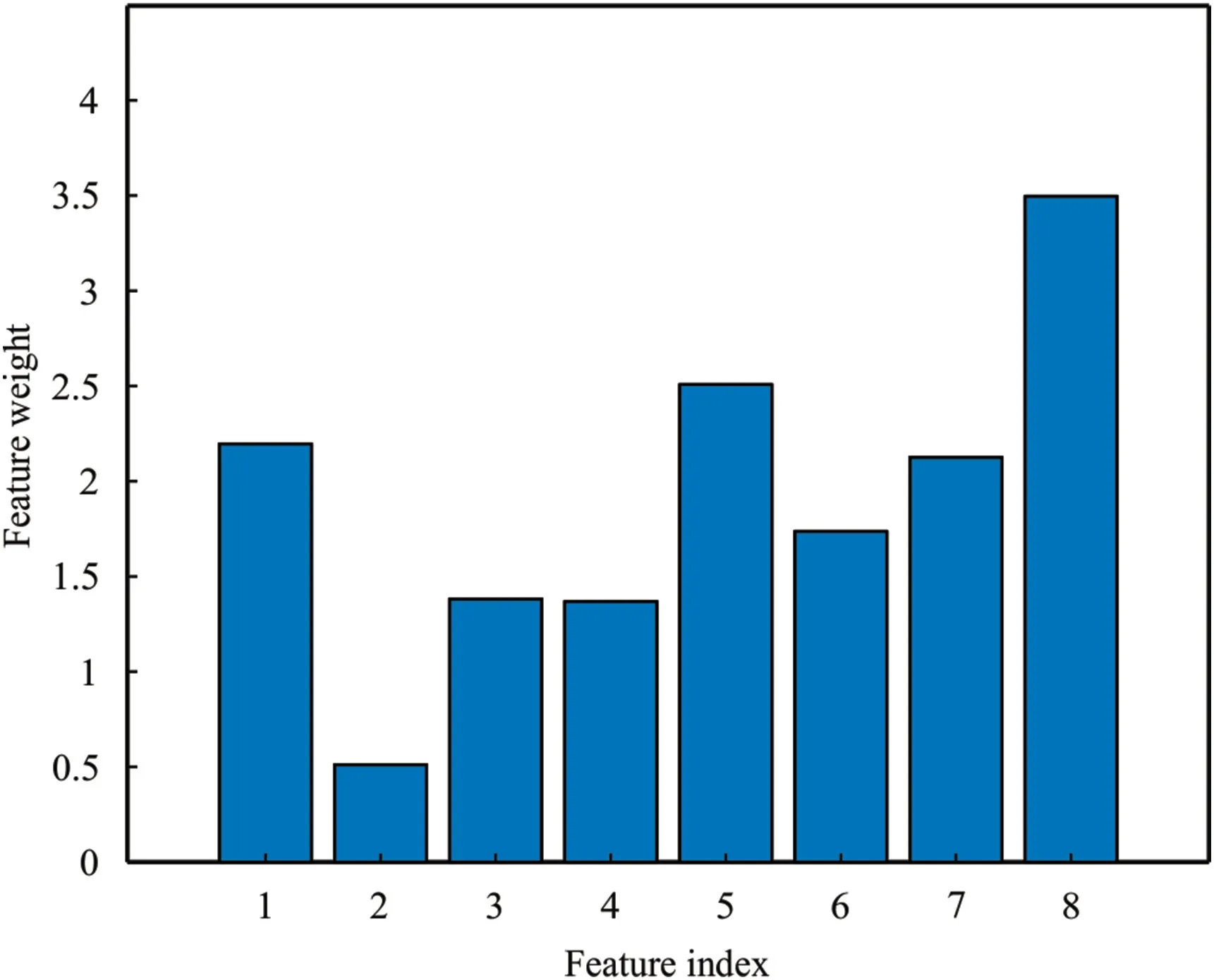
Fig.10.The value obtained using the NCA feature selection algorithm for each of the studied features.
For permeability modeling using selected features,80% of the data were designated as training and 20% as test data.Then,MLPNN with different structures was used to model the training data,which showed that the best structure for modeling permeability with selected properties is the use of an MLP-NN with two hidden layers,which are 3 and 5 neurons.They are in the first and second layers,respectively.
Fig.11 compares the results of three network training algorithms,Trainlm,Tgrainscg,and Trainrp.The Trainlm algorithm is a network training function that updates weight and bias values based on Levenberg-Marquardt optimization.The Levenberg-Marquardt optimizer function uses the gradient vector and the Jacobin matrix instead of the Hessian matrix.This algorithm is designed to work specifically with loss functions,which are defined as the sum of error squares.The trainscg algorithm updates weights and biases based on the scaled conjugate gradient method.SCG was developed by Müller.Unlike algorithms for conjugate gradients that require a line,this algorithm does not perform the search steps linearly,thus reducing computational time.The Trainrp algorithm also updates weights and biases based on the resilient backpropagation algorithm.This algorithm eliminates the effect of partial derivative size.In this algorithm,only the derivative symbol is used to determine the direction of weight updates,and its magnitude does not affect weight updates.It should be noted that the results of the implementation of the above algorithms in 10 consecutive iterations with the best results are drawn in this diagram.Considering RMSE as the evaluation criterion,it is clear that the Trainlm method has the lowest error rate among the described methods.Therefore,the mentioned method is reliable and can be used to implement the MLP neural network algorithm.
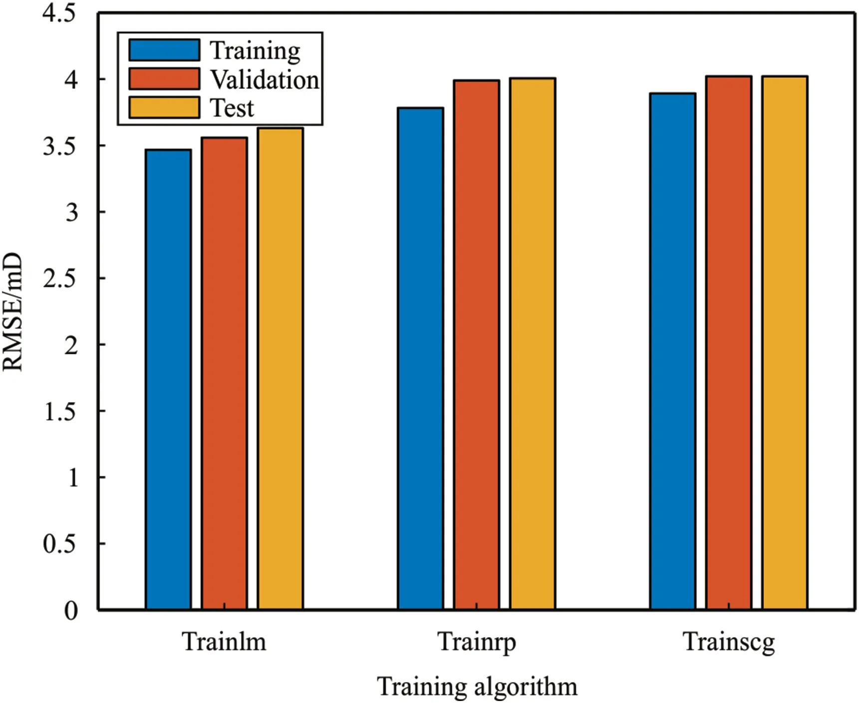
Fig.11.Comparing different training algorithms in the accuracy of MLP-NN.
The diagram of the mean square error(MSE)changes in epochs for the MLP method with the Levenberg-Marquardt optimizer has shown in Fig.12.As mentioned earlier,neural network architecture consists of 2 hidden layers with 3 and 5 neurons.In this method,the stop condition is considered not to improve the validation error rate in 6 consecutive repetitions,which finally ends the algorithm in 169 epochs.According to the figure,it is clear that at first,the MSE error decreased with a steep slope and then reached a fixed trend.Also,overfitting did not occur,and the best error rate in the validation step with this method is 11.8889.
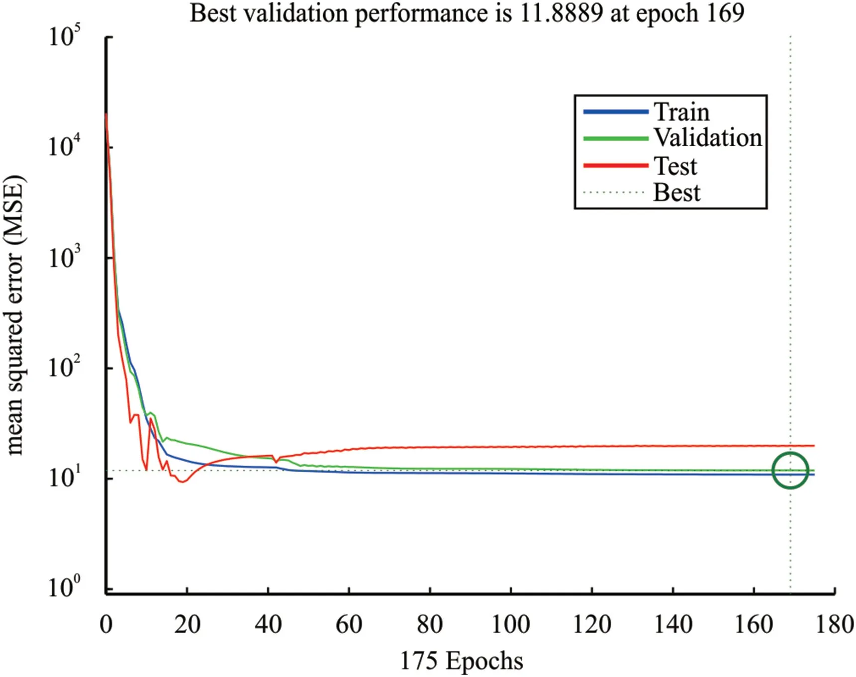
Fig.12.Changes of MSE for training,validation and test subsets at each iteration.
Fig.13 shows cross plots of measured and the predicted permeability of the rock for training,validation,and test and all data.The charts indicate a good forecasting trend,except for one outlier point,which can be seen in the training step.According to the graph from zero to the first half,the line graph y=t and the amount of permeability estimation are superimposed,however,in the second half,the estimated value is less than the actual value,so the underestimation has occurred.The correlation coefficient (R)values for train,test and validation steps are 0.99354,0.99578,and 0.99383,respectively,indicating that the MLP method is acceptable for predicting rock permeability.Outliers affect the amount of R,so We have also calculated the RMSE,which were equal to 4.0244,4.3603,and 4.9080 in train,validation,and test cases,which also indicates the reliability of this method.
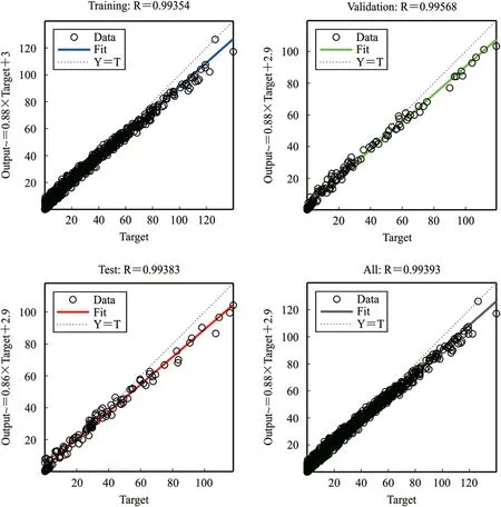
Fig.13.Crossplots of measured and predicted permeability for training,validation,test and all data.
Fig.14 illustrates the error histogram of the trained neural network with 20 bins for the three steps of train,validation,and test.As we can see,the orange line means the average accuracy in the middle of the chart is close to zero,and the curve has a normal distribution and is slightly skewed to the right.This indicates that the fitting error (error distribution of this method) is in an appropriate range.
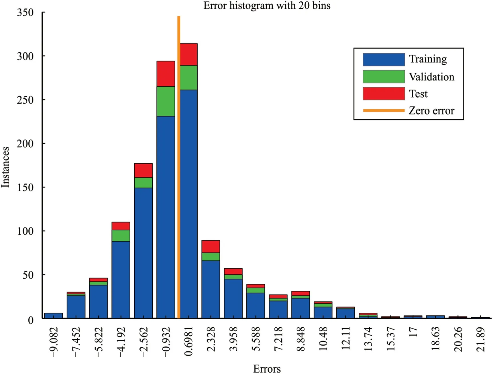
Fig.14.Error histogram for obtained results of training,validation and test subsets using simple MLP-NN model.
For permeability modeling with hybrid algorithms,it is necessary to determine the values of controllable parameters of the optimization algorithm.For this purpose,a sensitivity analysis was performed,the results of which are displayed in Table 4.
The measured and predicted values of rock permeability for three hybrid models which were introduced in this paper are shown in Fig.15 on both training and test data.The coefficient of determination (R2) expresses an alternative method to the RMSE(objective function of the model)for evaluating the accuracy of themodel prediction.R2is a statistical criterion that shows the ratio of variance for a dependent variable that is described by one or more independent variables in the regression model.IfR2=1 then the permeability of the rock is predicted without error by the selected independent variables.The higher this value,the lower the prediction error.The values ofR2on the training and test data for the three hybrid models(MLP-GA,MLP-PSO,and MLP-SSD)are given in Fig.15.These results are the best results of several sets of experiments in the 10-fold cross-validation method and also show that all of these methods have a high degree of correlation between the measured and predicted values.

Fig.15.Measured versus predicted values for rock permeability for three developed hybrid machine-learning models applied to the training and testing data subsets:(a)MLP-GA train data;(b) MLP-GA test data;(c) MLP-PSO train data;(d) MLP-PSO test data;(e) MLP-SSD train data;and,(f) MLP-SSD test data.
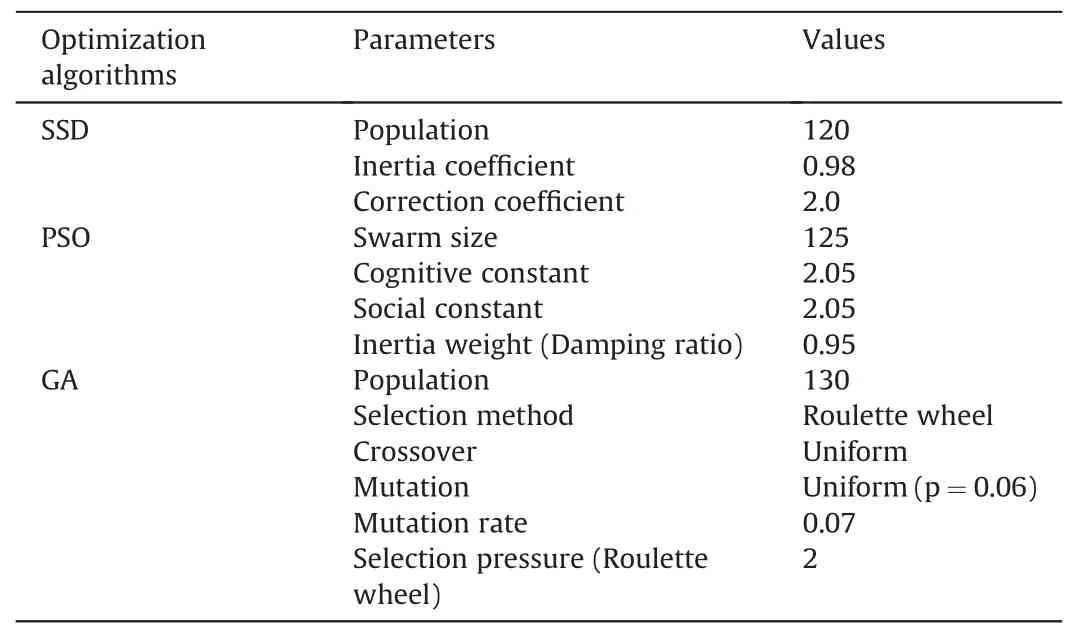
Table 4 Results of sensitivity analysis on the controllable parameters of optimization algorithms.
It is noteworthy that the introduced hybrid models have high accuracy in predicting the permeability of the rock (the ability of the rock to pass the fluid).The maximum value ofR2(0.9982) is obtained by the MLP-SSD algorithm,which represents the bestpredicted correlation performance for rock permeability.The second most accurate model is MLP-PSO withR2=0.9915,followed by MLP-GA with the lowest prediction(R2=0.9892)accuracy among these hybrid models.In addition,as shown in the figure,there is not much difference in accuracy between the training and test data,and therefore the model is not over-fitted and is reliable.
The difference between the predicted values and the measured values for the rock permeability in the developed models is shown in Fig.16.The horizontal axis represents the measured permeability,and the vertical axis represents the difference between the predicted and measured permeability,known as the residual error.Although this error cannot be a valid indicator for the predicted model,it provides an understanding of the predictive performance of the models used in the permeability of the rock.The smallest mean residual error is 0.119 for the MLP-PSO hybrid model,followed by the MLP-SSD and MLP-GA models with absolute residual error values of 0.1209 and 0.2108,respectively.In general,the developed hybrid models used to predict rock permeability have acceptable predictive performance and the amount of noise or irregularities is not significant.
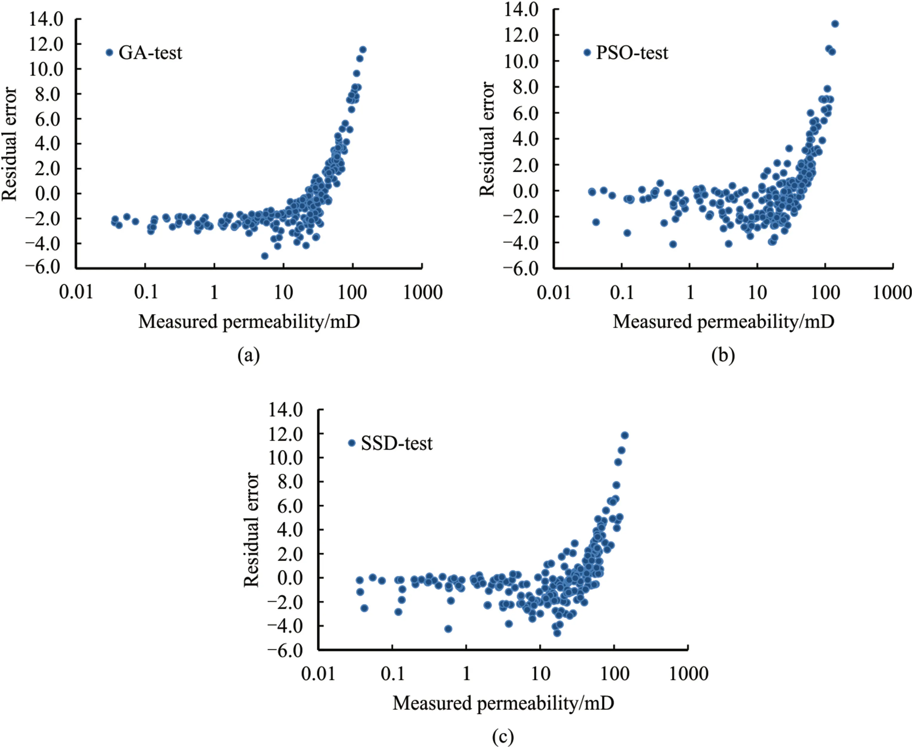
Fig.16.Relative deviations of measured versus predicted values of rock permeability (mD) for developed machine-learning models: (a) MLP-GA;(b) MLP-PSO;and (c) MLP-SSD.
The error histogram of hybrid models 1,2,and 3 are shown in Fig.17.According to the figures,it is clear that the means of the studied models are close to zero,and their standard deviation is insignificant compared to the maximum recorded value.The normal distributions,which are plotted on the error values obtained for all models,seem symmetrical and slightly skewed to the right.

Fig.17.Error (mD) histogram with fitted normal distribution (red line) for three hybrid machine-learning models: (a) MLP-PSO;(b) MLP-GA;and (c) MLP-SSD.
In evaluating forecast accuracy,we will gain a more accurate insight by comparing several separate statistical accuracies.In addition to the coefficient of determinationR2,the variance calculus,the root mean square error,the objective function of the hybrid models,and the performance index are used to evaluate the model's accuracy.The equations used for the calculation of these statistical parameters are shown in Appendix A.
The accuracy of the proposed models varies according to the small values of RMSE and the high values of VAF.Table 3 illustrates the values of RMSE,VAF,and PI for the models developed in this research.As can be seen,there is no significant difference between the accuracy obtained for the training and test data,so the introduced models are reliable,and no over-fitting has occurred during the training process.
According to Table 5,the RMSE value for MLP-SSD is smaller than the RMSE calculated for the test data of other hybrid models.In second place is the MLP-PSO method with RMSE=2.57 and VAF=99.15.It is followed by the MLP-GA model with the RMSE value of 2.89,which has the maximum absolute value of PI between the proposed methods.
Fig.18 illustrates the error changes in 10 runs with300 different iterations of SSD,PSO,and GA optimization algorithms in each run.In terms of the average changes,the GA optimization algorithm reaches the desired value of RSME in approximately 200 iterations.The SSD and PSO algorithms converge in 270 and 300 iterations,respectively.In addition,all the algorithms under study are convergent and will reach almost the same RMSE after a certain number of iterations.The only difference is that the GA method has less computational time than other methods.The training time of MLP network is significantly shorter than the hybrid algorithms.MLP-GA has the shortest training time among the hybrid algorithms.MLP-PSO is performing slightly faster than the MLP-SSD.Running the code on a system with 64.0 GB RAM and 2.4 GHz CPU(2 processors)resulted in 28 s,726 s,and 771 s calculation time for MLP,MLP-PSO,and MLP-SSD algorithms,respectively.
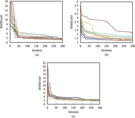
Fig.18.The convergence error for a) MLP-SSD b) MLP-PSO c) MLP-G.
5.Conclusions
This study employs intelligent hybrid methods to estimate the permeability of rock from other petrophysical features.Multilayer perceptron network was combined with three heuristic algorithms(SSD,GA,and PSO) to optimize the efficiency and improve the convergence of the networks.Petrophysical logs and data were collected from a well drilled into Fahlian formation in one of the Iranian southwestern fields.The outliers in the data were identified and removed and feature selection was carried out to enhance the accuracy of the network in predicting the permeability of the rock.The results show all the tested hybrid methods estimate the permeability with high accuracy.MLP-SSD method which was usedfor the first time in this study for estimation of permeability demonstrated slightly better results compared with other hybrid methods.MLP-GA was the least computationally expensive method among the examined networks.Overall,the excellent performance of the hybrid methods in the estimation of permeability for the case studied here indicates that such algorithms are applicable in highly heterogeneous formations.
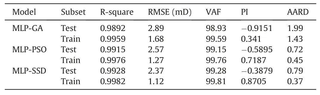
Table 5 Prediction accuracy statistical measures of permeability (mD) for three developed machine learning models.
6.Limitations and suggestions
The generated results in this study are limited to the Fahlian carbonate formation.Although we expect the model to work efficiently in other zones because of its excellent performance in a highly heterogeneous formation,still,it is advised to use the model with care in other formations and rocks.
Code and data availability
The developed MLP-SSD and MLP-PSO codes in MATLAB R2020b to produce this paper are available at https://github.com/mmehrad1986/Hybrid-MLP.
The used data in this study is not available because of respecting the commitment to maintain the confidentiality of the information.
Declaration of competing interest
The authors declare that they have no known competing financial interests to personal relationships that could have appeared to influence the work reported in this paper.
Appendix AEquations of the Statistical Parameters
whereyandzare real and predicted values of the dependent variable,andpis the number of dataset's records.
杂志排行

Petroleum的其它文章
- Super gas wet and gas wet rock surface: State of the art evaluation through contact angle analysis
- Petroleum system analysis-conjoined 3D-static reservoir modeling in a 3-way and 4-way dip closure setting: Insights into petroleum geology of fluvio-marine deposits at BED-2 Field (Western Desert,Egypt)
- Development and performance evaluation of a high temperature resistant,internal rigid,and external flexible plugging agent for waterbased drilling fluids
- Anti-drilling ability of Ziliujing conglomerate formation in Western Sichuan Basin of China
- Production optimization under waterflooding with long short-term memory and metaheuristic algorithm
- Investigation of replacing tracer flooding analysis by capacitance resistance model to estimate interwell connectivity