Production optimization under waterflooding with long short-term memory and metaheuristic algorithm

Cuthert Shng Wui Ng ,Ashkn Jhnni Ghhfrokhi ,Mend Nit Amr

a Department of Geoscience and Petroleum,Norwegian University of Science and Technology,Trondheim,Norway

b D′epartement Etudes Thermodynamiques,Division Laboratoires,Sonatrach,Boumerdes,Algeria

Keywords:Production optimization Numerical reservoir simulation Machine learning Long short-term memory (LSTM)Dynamic proxies Particle swarm optimization (PSO)

ABSTRACT In petroleum domain,optimizing hydrocarbon production is essential because it does not only ensure the economic prospects of the petroleum companies,but also fulfills the increasing global demand of energy.However,applying numerical reservoir simulation (NRS) to optimize production can induce high computational footprint.Proxy models are suggested to alleviate this challenge because they are computationally less demanding and able to yield reasonably accurate results.In this paper,we demonstrated how a machine learning technique,namely long short-term memory (LSTM),was applied to develop proxies of a 3D reservoir model.Sampling techniques were employed to create numerous simulation cases which served as the training database to establish the proxies.Upon blind validating the trained proxies,we coupled these proxies with particle swarm optimization to conduct production optimization.Both training and blind validation results illustrated that the proxies had been excellently developed with coefficient of determination,R2 of 0.99.We also compared the optimization results produced by NRS and the proxies.The comparison recorded a good level of accuracy that was within 3%error.The proxies were also computationally 3 times faster than NRS.Hence,the proxies have served their practical purposes in this study.

1.Introduction

In petroleum industry,reservoir management(RM)is one of the domains that has been emphasized by many oil and gas companies.According to Wiggins and Startzman [1],RM is termed as the employment of available technology,financial and labor resources to optimize the economic performance and recovery of a reservoir.They [1] further expounded that RM could be fathomed as a sequence of operations from its initial discovery of a reservoir to its final abandonment.In this case,production optimization is one of the pivotal parts in RM.Oil and gas companies attempt to optimize hydrocarbon production not only to fulfill the increasing demand for energy,but also to ensure their higher economic returns.One of the approaches of increased production is to perform waterflooding or water injection.Waterflooding is generally implemented to produce additional volume of hydrocarbon after primary recovery which relies upon natural mechanisms such as gas cap drive and gravitational drainage [2].Additionally,careful planning and implementation of waterflooding are important to avoid any unnecessary expenditure during the implementation phase.Hence,waterflooding optimization has been emphasized in the research field [3-7] for years to help the oil and gas companies to improve their application of this technique.

To be more precise,waterflooding optimization is considered as one of the engineering problems that requires some mathematical algorithms to come up with some design parameters,which either maximize or minimize any predefined objective function [2,8].Regarding this,these design parameters include well production rates,well injection rates,bottomhole pressure of well,initiation time of waterflooding,and so forth.More intriguingly,waterflooding problem can also be formulated into a multi-objective problem in which more than one objective function is optimized [9-11].This formulation provides more useful insights to the chemical or petroleum engineers as it has closer proximity to the real-life problem.Additionally,numerical reservoir simulation(NRS)is one of the most widely applied tools of reservoir modeling during the field development stage.NRS can be conveniently employed along with other algorithms to solve any problem related to production optimization.However,one of its drawbacks is that more computational effort is required if it is used to model a geologically sophisticated reservoir[12,13].This is because NRS uses mathematical equations and physics-based approach to model the flow of fluid in the subsurface.Thus,the computational time of the fluid flow modeling undeniably increases as the complexity of the reservoir modeled increases.Mitigating this computational challenge has been one of the most prevalent research topics.

Thanks to data-driven technology,the computational challenge can be alleviated.Data-driven technology is a framework that applies any input and output data provided to establish a relationship among them [13].A model that is yielded from this technology is known as “data-driven model”.In this aspect,the main building block of this technology is data.More importantly,machine learning (ML) is one of the techniques used for data-driven modeling.Examples of ML generally include artificial neural network,support vector machine,random forest,extreme gradient boosting,and so on.In addition,data-driven model has displayed its ability to be used as a proxy or surrogate model of NRS.Regarding this,a proxy or surrogate model in general acts as a substitute of NRS and is computationally faster and able to replicate the results of NRS within satisfied level of accuracy.In this context,Dr.Shahab Mohaghegh is one of the pioneers in the petroleum industry to have coined the term of smart proxy model(SPM).SPM is a proxy model that comprises an ensemble of numerous interlinked neuro-fuzzy systems,which are trained to understand the fluid flow behaviors from NRS[13,14].SPM has been demonstrated to be successful in different fields of application,including uncertainty analysis [15,16],CO2sequestration and utilization [17,18],history matching [19,20],waterflooding [21],and unconventional resources [22,23].Apart from these,there are other captivating literatures [24-33] discussing the use of ML-based models in the petroleum domains.These literatures in general also elaborated on the high applicability of ML techniques to be employed as a substitute of NRS.Nevertheless,one of the limitations of ML-based proxy modeling is the sufficiency of data.This is because the established ML-based model might not be able to“learn properly”without being supplied with sufficient data.However,when it is provided with too much data,this might undermine the significance of proxy modeling as a lot of simulation runs have to be performed.

Other than being used as proxy models,ML techniques have portrayed their value in the development of predictive models.In this case,Talebkeikhah et al.[34]successfully implemented seven ML methods,based on 1000 experimental points from some Iranian crude samples,to develop the predictive models of viscosity at reservoir conditions.These methods include radial basis function neural network,multilayer perceptron,support vector regression,adaptive neuro-fuzzy inference system,decision trees,and random forest.Besides that,Nait Amar et al.[35] illustrated how the best two out of various developed ML-based models were chosen and combined under the paradigm of committee machine intelligent system (CMIS) to develop a model that could forecast thermal conductivity of carbon dioxide.They further showed the use of weight average approach and group method of data handling (GDMH) to establish the CMIS models.A similar approach was employed and discussed by Mehrjoo et al.[36] to create a predictive model of interfacial tension of methane-brine systems at high pressure and salinity conditions.Also,based on 1985 experimental points,Nait Amar et al.[37] successfully applied gene expression programming to perform the modeling of density of binary and tertiary mixtures of ionic liquids and molecular solvents.

In this work,we have used an advanced ML technique that is long short-term memory(LSTM)to build two proxy models,which are correspondingly applied to predict field liquid production rate(FLPR) and field water cut (FWCT).It is essential to point out that the proxy models built here are considered as “dynamic proxies”,which are time-dependent.As Nait Amar et al.[24] stated,timedependent proxies offer higher flexibility in terms of application under time-dependent constraints.As the two abovementioned dynamic proxies were developed,they were coupled with particle swarm optimization (PSO) to conduct the waterflooding optimization.The details would be presented in the next few sections.After this introduction,the paper is followed by the theoretical framework that generally briefs the techniques involved and the general methodology used in this work.Thereafter,results and discussion about the main findings of this work are presented.The paper then ends with some conclusive remarks derived from this work.

2.Theoretical framework

2.1.Long short-term memory (LSTM)

LSTM is a more advanced version of recurrent neural network(RNN) that is developed to process sequential data,such as texts,sentences,and so on [38].A simple RNN is generally designed to preserve and deliver information from the current step to the next one [38].However,a simple RNN suffers the problem of vanishing gradient in which a long-term information cannot be fully utilized[39].Thus,large amount of previous information is unable to be stored to perform forecast within higher level of accuracy.To elude the problem of vanishing gradient,Hochreiter and Schmidhuber[39]built the LSTM in 1997.The fundamental topology of the LSTM used in this study is demonstrated in Fig.1.The mathematical formulation of LSTM is shown below:

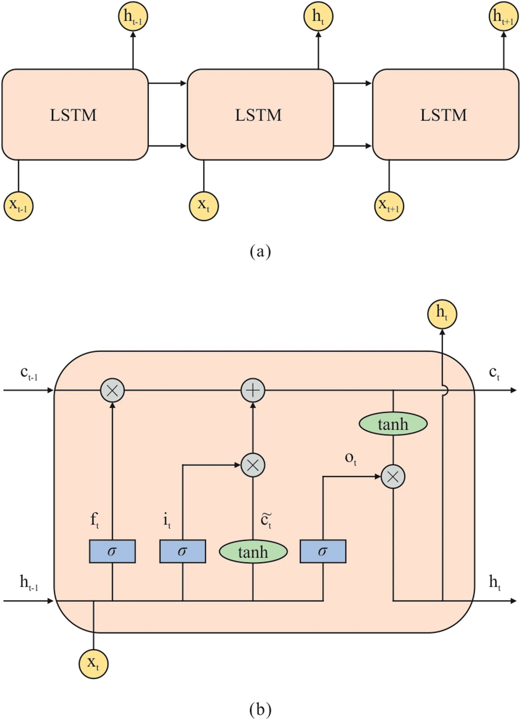
Fig.1.Architecture of Long short-term memory(LSTM):(a)general topology of LSTM.(b) detailed structure of LSTM.

The mechanism of LSTM revolves around a cell state ct.Around the cell state,information is either added or removed via three gates,for instance forget gate ft,input gate it,and output gate ot.These gates evaluate if the sequential input data should be retained to save pertinent information to the latter stages.Thereafter,according to Equation (1),the forget gate decides on the addition or omission of information.Regarding this,the information in terms of input and hidden state will be saved(removed)if ftis close to one(zero).Besides that,the input gate is calculated to update the cell state.Via this update,the evaluation of the importance of the input delivered to the next cell is done.Furthermore,the output gate computes the output for the hidden states based on equation(6).It can be noticed that the activation function and the recurrent activation function used in LSTM are respectively hyperbolic tangent function (indicated as tanh) and sigmoid function (denoted as σ).

2.2.Particle swarm optimization (PSO)

In 1995,Kennedy and Eberhart[40]established an optimization algorithm which was known as PSO.In this case,PSO is considered as an example of nature-inspired algorithms because it is formulated by simulating the behavior of flying stock of birds.Mathematically speaking,a swarm of particles indicates several possible solutions to an optimization problem.The status of each particle is computed according to its position and velocity.In this context,the dimension of both position and velocity is the same as the number of optimization parameters.In general,the algorithm commences through the random initialization of the position and velocity of each particle.A cost function,like mean squared error (MSE),is then employed to determine the fitness of each particle.After that,pbest and gbest are computed and saved to update the velocity at current iteration based on equation (7).In this context,pbest and gbest are found out for every iteration.pbest is the best position of a particle in the dimensional space and gbest is the overall best position of a particle hitherto in the whole swarm.Upon determining the velocity at next iteration,the position of a particle for the next iteration is updated as captured by equation(8).After a predefined number of iterations,each particle updates its position by minimizing the fitness value until the convergence of the optimal position occurs.

In equation (7),vjk，tcorresponds to the velocity of the jth particle at step t in kth dimension.xjk，tis its respective position.c1and c2correspondingly represent the cognitive and social learning factors that regulate the local and global search of the optimal solution.These parameters are selected by trial-and-error approach.r1and r2are random numbers extracted from uniform distribution of(0,1).ω is inertial weight that was suggested by Shi and Eberhart[41] to better handle the convergence issue.

Apart from PSO,we would like to reiterate that there are several other metaheuristic algorithms that can be employed to perform modeling and optimization tasks.Examples of these algorithms[42] include,but are not limited to,genetic algorithm,differential evolution,simulated annealing,and ant colony optimization.In this aspect,PSO has been selected due to its computational efficiency and perceivable concept as being briefed in the literature[43].Also,it has exhibited good results in some of our previous works[29,31,44].

2.3.Formulation of optimization problem and dynamic proxy

One of the most important perceptions about developing a proxy model is that it is an objective-oriented task.This implies that the background of the optimization problem must be clearly understood to provide better insights of proxy modeling.By perceiving the optimization problem,the modelers would know what variables or design parameters should be involved in creating the relevant proxies.Hence,formulation of optimization problem is indeed necessary in the development of proxies.In this work,the selected objective function is net present value (NPV),and it is mathematically shown in equation (9).

where u is the vector of optimization parameters,Qiis the field production (injection) rate at timestepiandPrepresents price or cost.The subscripts of o,w,and wi respectively indicate oil,water,and water injected.In this work,Pois 70 USD/bbl whereas both Pwand Pwiare 2 USD/bbl.Also,the optimization parameter used here is the field injection rate.Therefore,the optimization problem pertains to the adjustment of field water injection rate per 150 days for the period of 3000 days.Moreover,Δtiis the difference of time between current and previous timestep.Besides that,tiis the elapsed time from beginning until stepiandDis the reference time for discounting.Dis 365 days as interest rate has a unit of fraction per year and discounting of cash flow is done daily.The interest rate used here is 0.1 per year.

It is noticeable that the dynamic proxies developed here need to yield two parameters,which are field oil and water production rates(FOPR and FWPR).Therefore,by implementing LSTM method,we built two different dynamic proxy models,which respectively predict FLPR and FWCT at a specific timestep.Moreover,the input parameters are the number of days at every timestep i,ti;the harmonic mean of grid absolute permeability for every layer of formation,kharmonic;the standard deviation of grid absolute permeability for each formation layer,kStdDev;the permeabilities of completed grid blocks(injectors and producers),k{inj,prod};the field water injection rate,u;the output value at previous timestep,yi-1.The mathematical formulation of the proxies1The permeability refers only to the horizontal permeability,here.Also,the permeability in both x-and y-directions are the same.is illustrated in equation (10).The harmonic mean of permeability for every formation layer is given by equation (11).

whereLjrepresents the depth at the top of grid block j,kjrefers to the grid absolute permeability,and m denotes the number of grid blocks.Regarding the inputs of the permeabilities of completed grid blocks (injectors and producers),the reservoir model studied here is the “egg model” that was developed by Jansen et al.[45].There are 7 layers in the reservoir model with 8 injectors and 4 producers.To avoid the curse of dimensionality,the arithmetic mean of the permeability of the completed grid blocks for every well is calculated and this will yield 12 permeability variables.There are also 14 variables of kharmonicand kStdDevgiven egg model has 7 layers.In total,there are 29 input variables used to train the dynamic proxies.

About the geological properties of egg model,its permeability is heterogeneous whereas its porosity is homogeneous with a value of 0.2.The initial water saturation for each grid block is 0.1.The dimension of each block is 8 m×8 m×4 m with a total number of 60 × 60 × 7 (only 18533 grid blocks are active).The horizontal permeability distribution of egg model is illustrated in Fig.2.Refer to Jansen et al.[45] for the remaining details of the geological properties of this model.To be able to conduct the studies here,the control of both injectors and producers has been altered.In this aspect,the eight injectors are identical,and the rate is within the range of 40 m3/day and 100 m3/day.Hence,the optimization problem considering the constraint is summarized as shown below:

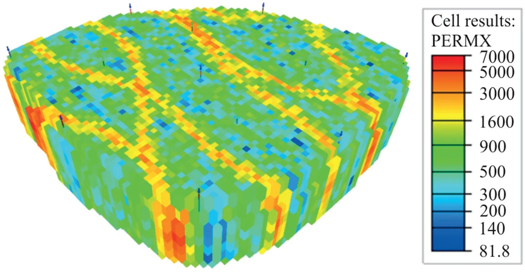
Fig.2.Permeability distribution of egg model.

2.4.Data preparation,neural network training,and blind validation procedure

After completing the formulation of optimization problem and dynamic proxy modeling,we have a clearer idea of input and output variable types.Thereafter,we employ the methodology discussed and used in Ref.[31] to conduct the proxy modeling.With respect to this,a database needs to be generated and formatted that can be used to train the dynamic proxies.To create this database,we generate 60 different injection schedules by employing three sampling techniques,such as Latin Hypercube Sampling [46],Hammersley Sequence Sampling [47],and Sobol Sequence Sampling [48].Each technique constitutes 20 schedules.Thereafter,each of the schedules is fed into the reservoir simulator to provide the necessary information to build the database.

For illustrative purposes,the summary of the database is presented in Table 1.It is essential to highlight that the statistical parameters provided in Table 1 are determined “categorically”.For instance,for the variable of kharmonic,the maximum and minimum values are determined by finding the highest and lowest values of all the 7 variables of kharmonic(knowing that there are 7 layers).By following this logic,the pertinent mean and standard deviation are computed.

Then,when the database is ready,it is normalized between 0 and 1 “categorically” using the following formula:

where Xnormalizedimplies the normalized value of Xnwhereas Xmaxand Xmincorrespondingly represent the maximum and minimum values of X.Then,the database was divided into training set(80%of the points),validation (10% of the data),and testing sets (the remaining 10%).Validation set is employed to prevent any overfitting issue during training whereas testing set is used to evaluate the predictability of the model prior to proceeding to blind validation phase.If excellent performance is illustrated during training,validation,and testing stages,then we would proceed to generate the database of blind validation.In this case,we reapply each of the three abovementioned sampling methods to respectively create additional 80 injection scenarios.Thereafter,we evaluate if the prediction performance of the dynamic proxies is within satisfied level of accuracy.Upon finishing the blind validation phase,the proxies are prepared for application.In this paper,we have utilized two statistical metrics to evaluate the training and prediction performance of the models,namely coefficient of determination and root mean squared error.The formula of each metrics is correspondingly displayed as Equations (14) and (15).

Table 1 Summary of database.

where Yiindicates the output value,the superscripts proxy and sim represent the proxy model and reservoir simulator model,respectively,is the mean value of the output,and n is the number of data points.

3.Results and discussion

Before proceeding to the results of our dynamic proxy models,it is essential to briefly explain that the trial-and-error approach has been implemented to determine the topology of our proxies.In this case,the dynamic proxy of FLPR has been built with one input layer,one hidden layer,and one output layer.There are 50 nodes used in the hidden layer.Besides that,the dynamic proxy of FWCT has the similar architecture as that of FLPR but with an additional hidden layer.Both hidden layers consist of 50 nodes.Besides that,one of the backpropagation algorithms,namely adaptive moment estimation(Adam),has been applied to train both proxies.Peruse King and Ba[49]for details.Pertaining to the parameters considered for Adam,the number of training iterations is 2000,the learning rate is 0.001,exponential decay rate for the 1st moment estimates is 0.9,that for the 2nd moment estimates is 0.999,and numerical stability is 10-7.

Fig.3 illustrates the cross plot between the actual values and the predicted values for both proxies of FLPR and FWCT.Based on this plot,it is deducible that albeit the proxy of FLPR slightly outperforms that of FWCT,both proxies have undergone an excellent training phase.This is further supported by the results of training,validation,and testing performance displayed in Table 2.With respect to this,it can be confirmed that the overfitting issue has been prevented as the validation performances of both proxies areas good as those of training.This also proves that both proxies have gone through a healthy trend of training.It is often important to ensure that the proxies have been trained “healthily”.Otherwise,the developed proxies will have a very weak predictability by only“memorizing”and being able to predict the data from the training set within satisfied level of accuracy.In addition,it is demonstrated that both proxies have good prediction ability as they have shown splendid testing results.Nevertheless,both proxies still must proceed to blind validation stage to further evaluate their predictability before being practically applied to perform optimization in this work.

Table 2 Training,validation,and testing performances of the dynamic proxies.

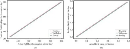
Fig.3.Cross plot between actual and predicted values considering training,validation,and testing sets: (a) FLPR.(b) FWCT.

To conduct the blind validation,three different sampling methods have been used to correspondingly create 80 additional injection schedules as mentioned earlier.Hence,each of these schedules will yield a set of performance metrics for each proxy.To provide a better evaluation of blind validation performance,the mean of the metrics for each sampling technique is shown instead in Table 3.Based upon the results,it can be inferred that both proxies have been successfully blind validated and are prepared to be used for optimization.However,for illustrative purpose,the blind validation results of one of the samples retrieved by using Latin Hypercube method are displayed in Fig.4.Although the blind validation dataset has not been used to develop the models,the models can still predict the outputs reasonably well.This further provides higher confidence regarding the integrity of the proxies built in this paper.

Table 3 Blind validation performances of the dynamic proxies considering three sampling techniques.

Fig.4.Blind validation of Latin Hypercube sample set 32 (out of 80): (a) FLPR.(b) FWCT.

As it has been explained,both proxies of FLPR and FWCT have been coupled with PSO to conduct the waterflooding optimization.In this aspect,the FWIR would be periodically tuned to maximize the NPV for a certain period of production.Regarding the parameters of PSO,the inertial weight is 0.8 whereas both the social and cognitive learning factors are 1.05.Also,the number of iterations is initialized to be 100 in tandem with 15 particle swarms per iteration.The case in which the optimization is done by applying both proxies,is termed as “dynamic proxies”.Thereafter,to assess the proximity of results of optimization,the optimized FWIRs resulted from the case of “dynamic proxies” are fed into the simulator to compute its respective NPV.Such case of optimization is known as“simulator-dynamic proxies” in this paper.To have a more comprehensive comparison,the reservoir simulator has also been coupled with PSO to conduct the optimization.This case is labeled as “simulator”.

Upon completing these three cases,the optimal NPV obtained from each case is recorded in Table 4.In general,it is noticeable that the proxies have illustrated practically accurate results.When comparing the NPVs of“simulator-dynamic proxies”and“dynamic proxies”,the error is calculated to be 2.6%.Furthermore,the error between “simulator” and “dynamic proxies” is determined to be 1.6%.For illustrative purpose,the optimized FWIRs derived from“simulator” and “dynamic proxies” are plotted in Fig.5.More interestingly,regarding the strength of the models,the computational time for “dynamic proxies” is about 4 h whereas that of“simulator” is about 12 h.Hence,the dynamic proxies are 3 times faster than the simulator for optimization in this study.This highlights the significance of the application of dynamic proxies.Tofurther check the integrity of these proxies,the plot of optimized field water (oil) production rates between “simulator-dynamic proxies” and “dynamic proxies” is illustrated in Figs.6-7.The respective statistical evaluation is also tabulated in Table 5.Based on these results,both proxies have practically served their purposes of application by reaching satisfied level of accuracy with less demanding computational effort.

Table 4 Optimal NPV considering three cases.

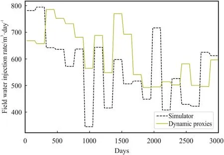
Fig.5.Optimized FWIRs derived from Simulator and Dynamic Proxies.

Fig.6.Optimized FWPR derived from Simulator-Dynamic Proxies and Dynamic Proxies.

Fig.7.Optimized FWOR derived from Simulator-Dynamic Proxies and Dynamic Proxies.

Nonetheless,there are a few limitations about the models developed in this work.As mentioned earlier,one of the limitations includes the application of the models.In this aspect,proxy modeling is an objective-driven task.Therefore,the established models can only be aptly employed to solve the optimization problem outlined.Besides that,there is a concern about the behavior of the training database as noise,which is an important issue to flow rate signal,is not considered in the data used.Hence,the models might not demonstrate high applicability when noisy data is introduced for optimization purpose.This is indeed part of the future works that is worth investigating.

Table 5 Statistical evaluation of optimized FWPR and FOPR.

4.Conclusions

In this study,we applied the LSTM approach to develop two dynamic proxies,which correspondingly could predict FLPR and FWCT based upon a 3D reservoir model known as the“Egg Model”.One of the main objectives of this investigation was to study the applicability of LSTM to be employed as proxy models for production optimization.According to the training and blind validation results,it could be deduced that these two proxies could accurately emulate the outputs yielded by the reservoir simulator.Moreover,we coupled these dynamic proxies with PSO to conduct the optimization.From the results of optimization and comparative analysis,the dynamic proxies were able to yield optimal results close to simulator only within 3% error,but 3 times faster.This finding further highlights the significance of dynamic proxies in terms of application.Although these proxies are case-dependent,they have excellently served their purpose of use in this study.Besides that,these summarized findings also confirm the cogency of the methodology used to establish these dynamic proxies.Finally,we also believe that there is still room for improvement of the methodology discussed in this paper.One of them includes the consideration of noise-handling ability as highlighted earlier.Besides that,the introduction of decision variables with higher dimensionality and the application of multi-objective optimization are parts of possible future studies.As the methodology achieves a satisfactory level of maturity,its potential use can later be extended to optimization of CO2storage and/or EOR.

Declaration of interest statement

The authors declare that they have no known competing financial interests or personal relationships that could have appeared to influence the work reported in this paper.

Acknowledgement

This research is a part of BRU21 -NTNU Research and Innovation Program on Digital Automation Solutions for the Oil and Gas Industry (www.ntnu.edu/bru21).