The Smoothing Newton Method for NCP with P0-Mapping Based on a New Smoothing Function

MA Changfeng(马昌凤),WANG Ting(王婷)

(1.Key Laboratory of Digital Technology and Intelligent Computing,School of Big Data,Fuzhou University of International Studies and Trade,Fuzhou 350202,China;2.School of Mathematics and Statistics,Fujian Normal University,Fuzhou 350117,China)

Abstract: The nonlinear complementarity problem (NCP) can be reformulated as the solution of a nonsmooth system of equations.By introducing a new smoothing function,the problem is approximated by a family of parameterized smooth equations.Based on this smoothing function,we propose a smoothing Newton method for NCP with P0-mapping and R0-mapping.The proposed algorithm solves only one linear equations and performs only one line search per iteration.Under suitable conditions,the method is proved to be globally and local quadratically convergent.Numerical results show that the proposed algorithm is effective.

Key words: Nonlinear complementarity problem;Smoothing Newton method;Smoothing function;Global convergence;Local quadratic convergence

1.Introduction

We consider the nonlinear complementarity problem(NCP),to find a vector(x,y)∈R2nsuch that

whereF: Rn →Rnis a continuously differentiable mapping,(x,y) is short for (xT,yT)T.IfF(x) is an affine function,then NCP reduces to a linear complementarity problem (LCP).

NCP has many applications in economics and engineering[5−6].Recently,there has been an increasing interest in solving the NCP by using smoothing methods.Roughly speaking,a smoothing method uses a smoothing function to approximate NCP via a family of parameterized smooth equations,solves the smooth equations approximately at each iteration,and refines the smooth approximation as the iterate progresses toward a solution of NCP.It is evident that smoothing functions play an important pole in smoothing methods.Up to now,many smoothing functions have been proposed: the Kanzow smoothing function[7],Engelke-Kanzow smoothing function[8],and so on.

It is well known that anx ∈Rnsolves(1.1)if and only if it solves the following nonsmooth equations[1−4]:

where the plus function [·]+is defined by

The plus function is applied to each component ofx.In this sense,the plus function plays an important role in mathematical programming.But one big disadvantage of the plus function is that it is not smooth because it is not differentiable.Thus numerical methods that use gradients cannot be directly applied to solve a problem involving a plus function.In this paper,we use a smoothing function approximation to the plus function.With this approximation,many efficient algorithms can be easily employed.We are interested in smoothing method.

The idea of using smooth functions to solve the nonsmooth equation reformulation of complementarity problems and related problems has been investigated actively.[9]Recently,there have been strong interests in smoothing Newton methods for solving the complementarity problem.[21−27]Note that some of them,ZHANG and GAO[21]propose a one-step smoothing Newton method for solving theP0-LCP based on Kanzow’s smoothing function.Their smoothing Newton method solves only one linear system of equations and performs only one line search at each iteration.It is proved that their proposed algorithm has global convergence and local quadratic convergence in absence of strict complementarity assumption at theP0-LCP solution.Later,they extend this method to the NCP based on the smoothing symmetric perturbed Fischer function[21]and the algorithm also has global convergence and local quadratic convergence without strict complementarity assumption.This algorithm has strong convergence results under weaker conditions and has a feature that the full stepsize of 1 will eventually be accepted.Motivated by the feature of this algorithm,in this paper,by using a new smoothing function approximation to the plus function above mentioned and modifying the algorithms in[21],we propose a smoothing method for NCP with aP0-mapping andR0-mapping.Compared to the algorithm in [21],our method has all their properties and has the following nice features: Our algorithm is simper and the fast step in our algorithm keeps the local quadratic convergence.

We establish the global linear and local quadratic convergence of the algorithm under suitable assumptions.Lastly,we give some numerical results which show that our method is efficient.For any (x,y)∈R2n,µ >0,our smoothing method for NCP is based on the following equation

whereµis a smoothing parameter.It is easy to show that

This paper is organized as follows.In Section 2,we study a few properties of the smoothing function.In Section 3,we give a one-step smoothing Newton method and the global linear convergence.The local quadratic convergence of the algorithm are discussed in Section 4.Preliminary numerical results are reported in Section 5.

In our notation,all vectors are column vectors,Rndenotes the space ofn-dimensional real column vectors,anddenotes the nonnegative [respectively,positive]orthant in Rn.For convenience,we also write (uT,vT)Tas (u,v) for any vectorsuandv.We denoteI={1,2,···,n}.For any continuously differentiable function

we denote its Jacobian by

where∇gidenotes the gradient ofgifori=1,2,···,n.

2.Properties of the new Smoothing Function

In this section,we mention some properties of the new smoothing function.

Lemma 2.1Let the smoothing functionϕ(µ,t) be defined by (1.5).We have the following results.

Lemma 2.2For anyµ1≠µ2∈R+,we have

ProofWithout loss of generality,we assume that 0≤µ1<µ2.

The proof is completed.

For any (x,y)∈R2,from the smoothing functionϕ(µ,·) defined by (1.5),we can obtain that

By simple calculation,we have

It is not difficult to see thatare continuous withµ>0.Then,from (2.1)-(2.3),we have the following results.

Lemma 2.3For any (µ,x,y)∈R++×R2,we have

Lemma 2.4FunctionH(µ,x,y) is continuously differentiable on R++×Rn×Rnand

whereIdenotes then×nidentity matrix and

3.Algorithm and Global Linear Convergence

Now we give the algorithm and some preliminaries that will be used throughout this paper.

Algorithm 3.1(One-step smoothing Newton method)

Step 0 Initialization.Chooseσ ∈(0,0.5],α ∈(0.5,1),δ ∈(0,1),ε≥0.Take an arbitrary vectorz0:=(µ0,x0,y0)∈R++×R2n.Chooseγ ∈[1,∞) such that‖H(z0)‖2/γ <1 andµ0/γ <1.Sete1:=(1,0,···,0)T∈R2n+1andk:=0.

Definition 3.1A mappingF:Rn →Rnis said to be a

1)P0mapping if for allx,y ∈Rn,x/=y,there exists an indexi ∈Isuch thatxi≠yiand

Lemma 3.1LetH(z) :=H(µ,x,y) be defined by (1.3).For anyz:=(µ,x,y)∈R++×R2n,define the level set

wherez0is given in Algorithm 3.1.Then,for anyµ2≥µ1>0,the set

is bounded.Furthermore,for anyµ>0,the setLµ(z0) defined by (3.4) is bounded.

ProofBy Lemma 2.2,for all (x,y)∈Lµ(z0,µ1,µ2),we have

where the second inequality follows from the relation ofG(µ,x,y) andΦ(µ,x,y).Thus,‖G(0,x,y)‖1is bounded.On the other hand,by‖min{x,F(x)}−min{x,y}‖1≤‖y −F(x)‖1,we have

where the first equality follows from min{x,y}=x −[x −y]+,(1.4) and Lemma 2.1 (ii),and the last inequality follows from the above deduction.So we have

By the above inequality,for any (x,y)∈Lµ(z0,µ1,µ2),‖min{x,F(x)}‖1is bounded.By Proposition 3.12 in [10],ifFis anR0function,then{x}is bounded if‖min{x,F(x)}‖1is bounded.BecauseF(x) is continuous and‖y −F(x)‖1≤‖H(µ,x,y)‖1≤‖H(z0)‖1,we obtain that{y}is bounded if (x,y)∈Lµ(z0,µ1,µ2).Then the setLµ(z0,µ1,µ2) is bounded.This completes the first part of the lemma.The boundedness ofLµ(z0) with anyµ>0 is the immediate corollary of the first part.

Lemma 3.2IfFis aP0mapping,then Algorithm 3.1 is well defined and generates an infinite sequence{zk=(µk,xk,yk)}withµk ∈R++andµk ≥σkµ0for allk >0.If for anyµ>0,(xk,yk)∈Lµ(z0),then we can show that (xk+1,yk+1)∈Lµ(z0) for allk >0.

ProofFrom Lemmas 2.3 and 2.4,we can know that

which imply thatDxand−Dyare positive diagonal matrices for any (µ,x,y)∈R++×R2n.SinceFis aP0mapping,thenF′is aP0matrix for anyx ∈Rn(see [11],Lemma 5.4).Thus,the matrixH′is nonsingular for anyµ>0 (see [12],Lemma 4.1).So the system (3.1) is well defined and has a unique solution.On the other hand,we can show that the backtracking line search (3.3) terminate finitely.From (3.1),we can obtain that

Therefore,for anyλ ∈(0,1]we obtain that

Thus,for anyλ ∈(0,1],by differentiability ofH,and combining (3.5),(3.6) andσk=‖H(zk)‖2min{1,‖H(zk)‖2}/γ,we have

It means that exists a constant∈(0,1]such that

holds for anyλ ∈(0,].This indicates that Step 3 of Algorithm 3.1 is well defined at thekth iteration.Therefore,by (3.5) and Steps 2-3,we haveµk+1=σkµ0>0 orλk ∈(0,1]andµk+1=µk+λk∆µk=(1−λk)µk+λkσkµ0>0.Thus,fromµ0>0 and the above statements,we obtain that Algorithm 3.1 is well defined and generates an infinite sequence{zk=(µk,xk,yk)}withµk ∈R++and we can easily obtainµk ≥σkµ0for allk >0.

Since (xk,yk)∈Lµ(z0),if Steps 2 is accepted,then from (3.2) andσ ∈(0,0.5),we can know that

Otherwise,we obtain that (3.3) holds.We have

which indicates that (xk+1,yk+1)∈Lµ(z0).We complete the proof.

The following theorem gives the global convergence of Algorithm 3.1 and the boundedness of the iteration sequence generated by Algorithm 3.1.

Assumption 3.1The solution set of NCP (1.1) is nonempty and bounded.

Theorem 3.1Suppose thatFis aP0function,and assume that the sequence{zk}is generated by Algorithm 3.1.The following three statements are valid.

(a) limk→∞‖H(zk)‖2=0 and limk→∞µk=0.

(b) Every accumulation point of the sequence{(xk,yk)}is a solution ofNCP(F).

(c) If Assumption 3.1 is satisfied,then the sequence{(xk,yk)}is bounded.

Proof(a) LetK1andK2be the sets of iteration indexksuch that the next iteratek+1 is obtained through Step 2 and step 3,respectively.(a) can be proved as follows:Case 1 IfK1is infinite,from (3.2) andσ ∈(0,0.5],we can know that

Formµk=σkµ0and (3.10),we have limk(∈K1)→∞µk=0.

Case 2 Suppose that the setK1is finite,thenk ∈K2for allksufficiently large.In the following we assume on the contrary that

From (3.6) and Lemma 3.2,we obtain that

whereσ∗=Hmin{1,H}/γ.Then,by Lemmas 3.1,3.2,we obtain that the sequence{(xk,yk),k ∈K2}is bounded.Thus,{zk,k ∈K2}is bounded.Subsequently if necessary,we may assume that there exists a pointz∗=(µ∗,x∗,y∗)∈R++×R2nsuch that

It is easy to see that

From‖H(z∗)‖2>0,we have limk→∞λk=0,thus,the stepsize:=λk/δdoes not satisfy the line search criterion (3.3) for any sufficiently largek;i.e.,the following inequality holds:

for any sufficiently largek,which implies that

Fromµ∗>0,we know thatH(z) is continuously differentiable atz∗.Letk →∞,then the above inequality gives

In addition,by taking parts of the limit on (3.1),we have

Combining (3.11) with (3.12) we have

which contradicts the fact thatδ ∈(0,1) andµ0/γ <1.This implies thatH(z∗)=0.Thus,µ∗=0 by the definition ofH(z).

In addition,by (3.3),(3.2) and Lemma 3.2,we obtain that{‖H(zk)‖2}and{µk}are monotonically decreasing.Therefore,putting together Case 1 and Case 2,we can know that statement (a) is true.

(b) Recalling the definition ofH(z) and limk→∞‖H(zk)‖2=0,a simple continuity argument implies that every accumulation point of the sequence{(xk,yk)}is a solution of NCP.

(c) Similar to the proof of Theorem 3.6 (b) in [20],we can easily obtain that (c) holds.

4.Local Quadratic Convergence

In order to discuss the local quadratic convergence of Algorithm 3.1,we need the concept of semismoothness,which was introduced originally by Mifflin[13]for functionals.QI and SUN[14]extended the definition of semismooth function to a vector-valued function.A locally Lipschitz functionF:Rm1→Rm2,which has the generalized Jacobian∂F(x)as in Clarke[15],is said to be semismooth atx ∈Rm1if limV ∈∂F(x+th′), h′→h, t↓0{V h′}exists for anyh ∈Rm1.F(·) is said to be strongly semismooth atxifFis semismooth atx,and for anyV ∈∂F(x+h),h →0,it follows that

Lemma 4.1[14]Suppose thatΨ:Rn →Rmis a locally Lipschitzian function.Then

(a)Ψ(·)has generalized Jacobian∂Ψ(x)as in[15].AndΨ′(x;h),the directional derivative ofΨatxin the directionh,exists for anyh ∈RnifΨis semismooth atx.Also,Ψ:Rn →Rmis semismooth atx ∈Rnif and only if all its component functions are.

(b)Ψ(·) is strongly semismooth atxif and only if for anyV ∈∂Ψ(x+h),h →0,

Suppose thatz∗is an accumulation point of the sequence{zk}generated by Algorithm 3.1.Then,the assumptions made in Theorem 3.1 indicate thatH(z∗)=0 and (x∗,y∗) is a solution ofNCP(F).Since a vector-valued function is strongly semismooth if and only if all its component functions are strongly semismooth,by Lemma 4.1,we obtain the following lemma.

Lemma 4.2Let functionΦandHbe defined by (1.4) and (1.3),respectively.Then

(a)Φ(·,·,·) is strongly semismooth on R+×R2n.

(b)IfF′(x)is Lipschitz continuous on Rn×n,thenHis strongly semismooth on R+×R2n.

ProofIt is not difficult to show thatc −d,(c −d)2is a strongly semismooth for all(c,d)∈R2.By recalling the definition ofΦand the fact that the composition of strongly semismooth functions is strongly semismooth,we obtain immediately thatΦ(·,·,·)is strongly semismooth at all points R++×R2n,we prove (a).IfF′(x) is Lipschitz continuous on Rn×n,thenxi −Fi(x),(xi −Fi(x))2are all strongly semismooth on Rnfor alli ∈I.It is easy to see from Lemma 4.1 that (b) holds.

Assumption 4.1F′(x) is Lipschitz continuous on Rn×n.

Theorem 4.1Assume that Assumptions 3.1 and 4.1 are satisfied andz∗=(0,x∗,y∗)is an accumulation point of the infinite sequence{zk}generated by Algorithm 3.1.If allV ∈∂H(z∗) are nonsingular,then the whole sequence{zk}converges toz∗and the relationshold for all sufficiently largek.

ProofIt follows from Theorem 3.1 thatH(z∗)=0.Because allV ∈∂H(z∗) are nonsingular,then for allzksufficiently close toz∗,we have

whereC >0 is some constant.By Lemma 4.2(ii),we know thatH(z)is strongly semismooth atz∗.Hence,for allzksufficiently close toz∗,we have

On the other hand,we know thatH(z) is strongly semismooth atz∗which implies thatH(·)locally Lipschitz continuous nearz∗,that is,for allzksufficiently close toz∗,we have

Similar to the proof of Theorem 3.1 in [16],for allzksufficiently close toz∗,we get

Then,becauseH(z)is strongly semismooth atz∗by Lemma 4.2,H(z)must be local Lipschitz.

Therefore,for allzksufficiently close toz∗,we obtain that

In view of the updating rule in Step 2 of the smoothing Newton method,(4.6) implies that the smoothing Newton method eventually executes the fast step only forksufficiently large,i.e.,there exists an indexk0such thatk ∈K1and=zkfor allk ≥k0.Therefore,for allk ≥k0,we have

which,together with (4.6),implies

Then,for allzksufficiently close toz∗,we haveµk+1=.The whole proof is completed.

5.Numerical Experiment

In this section,we test our algorithm on some typical test problems.The stopping criterion we used for our algorithm is

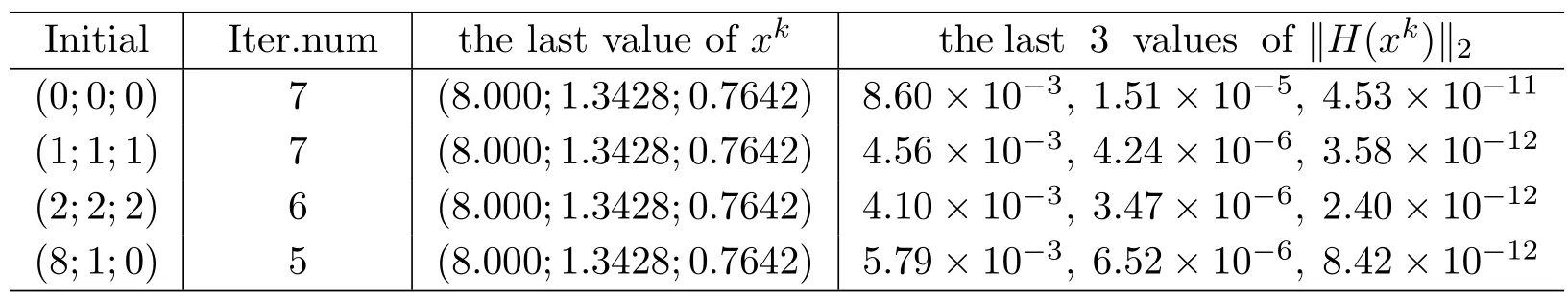
for someε>0.Throughout the numerical experiments,the parameters used in the algorithm areε=10−10,σ=0.5,δ=0.1,µ0=10−2,γ=‖H(z0)‖2/µ0andα=0.95,and sety0=F(x0).All the programming is implemented in MATLAB 7.1.The test problems are introduced as follows: In the first two linear test problems,we have the formF(x)=Mx+qand choose the initial pointx0=(1,1,···,1)T.We summarize the results of our algorithm for several values of the dimensionnin Table 1 and Table 2,respectively.In the last three nonlinear test problems,we choose difference initial points and the numerical results are listed in Table 3,Table 4 and Table 5,respectively.

LCP 1This linear complementary problem is one for which Murty has shown that principal pivot method I is known to run in a number of pivots exponential in the number of variables in the problem (see [17]),where

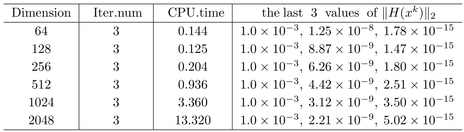
Tab.1 LCP1 Numerical results

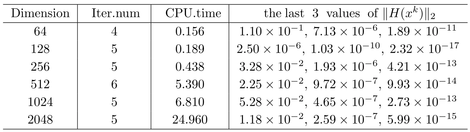
Tab.2 LCP2 Numerical results

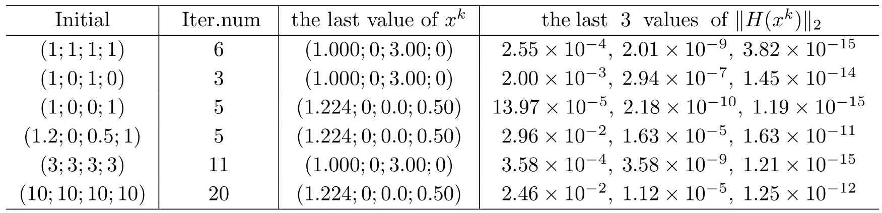
Tab.3 NCP1 Numerical results

Tab.4 NCP2 Numerical results

Tab.5 NCP3 Numerical results

Tab.6 Results of our algorithm by random initial points

LCP 2This is a linear complementarity problem,where

NCP 1This problem is a nonlinear complementarity problem from Kojima-Shindoet[18]

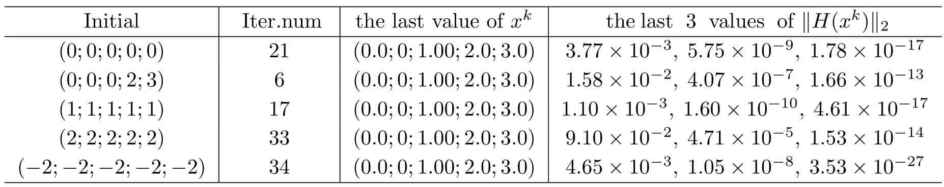
NCP 3This problem is a nonlinear complementarity problem from Kanzow(see [19]).It is obtained by five different definitions,where

From Tables 1-5,we see that the algorithm can solve these problems efficiently.From Column 4 of the five tables,we know that‖H‖2tends to 0 rapidly at the end of the algorithm.This shows the quadratic convergence behavior of our method.

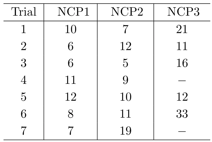
To illustrate the stability of our algorithm,we use the algorithm to solve problems NCP1,NCP2 and NCP3 for the initial pointx0which is produced randomly in (0,10).The number of the iterations is listed in Table 6.

6.Conclusions

Based on the ideas developed in smoothing Newton methods,we approximated the solution of the equivalent system of nonsmooth equations of nonlinear complementarity problem withP0-function andR0-function by making use of a new smoothing function.Then we presented a so-called one-step smoothing-type algorithm to solve the parameterized smooth equations.We have shown that Algorithm 3.1 converges globally and has local quadratic convergence result if the NCP(F) (1.1) satisfies a non-singularity condition andF′(x) is Lipschitz continuous on Rn×n.Numerical experiments show that the algorithm is efficient.Furthermore,these experiments demonstrate the quadratic convergence.