An approach for simulating the air brake system of long freight trains based on fluid dynamics
2023-06-14XinGeQinghuaChenLiangLingWanmingZhaiKaiyunWang
Xin Ge · Qinghua Chen · Liang Ling ·Wanming Zhai · Kaiyun Wang,2
Abstract Air brake systems are critical equipment for railway trains,which affects the running safety of the trains significantly.To study air braking characteristics of long freight trains,an approach for simulating air brake systems based on fluid dynamics theory was proposed.The structures and working mechanisms of locomotive and wagon air brakes are introduced,and mathematical models of the pipes,brake valves,reservoirs or chambers,cylinders,etc.,are presented.Besides,the dynamic motions of parts in the main valve are considered.The simulation model of the whole air brake system is then formulated,and the solving method based on the finite-difference method is used.New efficient pipe boundary conditions without iterations are developed for brake pipes and branch pipes,which can achieve higher computational efficiency.The proposed approach for simulating the air brake system is validated by comparing with published measured data.Simulation results of different train formations indicate that models that consider the dynamic behavior of brake pipes are recommended for predicting the characteristics of long trains under service braking conditions.
Keywords Air brake system · Fluid dynamics · Railway train · Boundary condition · Simulation
1 Introduction
The air brake system is a fundamental piece of equipment for railway trains,which plays an important role in speed regulation during routine operations and the quick brake stop under emergency conditions.For conventional long freight trains,the performance of the air brake system affects intrain forces remarkably,which further influences the running safety of trains [1–3].Due to the large scale of the system,the cost of a full-scale test platform is high,and numerical simulation techniques are widely adopted to study air brake systems.
According to Refs.[4,5],air brake models can be classified into empirical models,fluid dynamics models,and fluid-empirical dynamics models.Empirical models are established based on measured data of the air brake system without the consideration of fluid dynamics principles.For practical application scenarios that do not concern detailed characteristics of the air brake system,such as the headway design,signaling design,and braking distance calculation,the brake forces can be simplified as equivalent constant values [4].In train dynamic performance simulations,the lookup table models and fitting formula models are commonly used empirical models.The look-up table models based on interpolations or extrapolations of measured data can reflect detailed characteristics of the air brake system,such as the maximum pressure,pressure ascending time,brake delay,and pressure variations caused by quick service [6,7].The fitting formula models use mathematical functions,such as the power functions,natural exponential functions,and polynomial functions,to fit measured data,and the models consider the characteristics of the air brake system by introducing a set of control parameters [8–12].Empirical models are relatively simple and have high computational efficiency,but the models depend on the measured data excessively.Therefore,the fluid dynamics models following fluid dynamics principles are necessary for improving the air brake system or predicting its characteristics.
Air flows in brake pipes or branch pipes are fundamental parts of fluid dynamics models.Funk and Robe [13] presented a line-chamber model in which the pipe is modeled using the continuity equation and momentum equation,and the pipe wall friction is considered according to the Darcy–Weisbach equation.This model can reflect the fundamental mechanism of the air brake system and has been widely used in fluid dynamics models.Abdol-Hamid [14]extended Funk and Robe’s work to establish the simulation model of the whole air brake system,in which the branch pipes are modeled as additional volumes of the brake pipes,and the air leakage of the pipe is also taken into account.Based on Abdol-Hamid’s work,Specchia et al.[15,16]developed the Analysis of Train/Track Interaction Forces(ATTIF) software package.Focusing on Indian air brake systems with twin pipes and graduated-release features,Murtaza and Garg [17] established the simulation model based on Funk and Robe’s model.Pugi et al.[18] developed a parametric library for the simulation of UIC standard air brake systems based on the MATLAB-Simulink platform.Cantone et al.[19],Piechowiak [20,21],and Wei et al.[22]improved the classical pipe model based on the isothermal assumption and developed advanced pipe models that consider energy exchanges of the system.
Apart from the models considering the continuous flow of pressurized air in the pipe,there are some lumped parameter models of pipes.Belforte et al.[23] developed equivalent lumped parameter models of brake pipes by referring to electrical theories.Bharath et al.[24] and Teodoro et al.[25]presented a lumped model in which the pipes were modeled as a series of reservoirs connected via orifices.To solve the pipe models,the finite-difference method,finite element method,and method of characteristics are frequently used in simulations [4,26].The main difference between fluid dynamics models and empirical-fluid dynamics models lies in the brake valve models.The former models generally model the brake valve as fixed and variable volumes connected by orifices or pipes,considering the valve motions and interconnection logics [4,25,27],while the latter models empirically determine brake cylinder pressures or brake forces according to the brake pipe pressure signal [19,23].Fluid-empirical dynamics models are widely adopted in realtime simulation models to balance the model accuracy and computational efficiency.With the application of the parallel computing technique,the detailed fluid dynamics models can also achieve real-time simulation [28–30].
Previous studies have established train air brake simulation models using commercial software packages or in-house code.However,the low computational efficiency of commercial software cannot satisfy the demand for large-scale simulation,and models by in-house code are difficult to realize due to the complicated solution method and boundary conditions.The motivation of this paper is to propose a simplified approach to realize modeling and solving the air brake system based on fluid dynamics theory.Simple pipe boundary conditions without iterations are developed for brake pipes and branch pipes,which can simplify the programming process and achieve high computational effi-ciency compared to the commonly used method of characteristics.Taking the common air brake system in Chinese heavy-haul trains as an example,this paper has systematically introduced the structural composition and the working mechanism of the automatic air brake system.Then,the mathematical models of locomotive and wagon air brake systems are presented.Finally,the whole air brake system simulation model is developed,and the finite differencebased solving method as well as the pipe boundary conditions are illustrated.The model is further validated,and the characteristics of different train formations are also simulated and discussed.
2 Train air brake system
The air brake system of a long freight train is generally composed of electronically controlled pneumatic brake subsystems for locomotives and a series of fully air-controlled pneumatic brake subsystems for wagons,and all air brake subsystems of locomotive and wagons are serially connected through hoses,as shown in Fig.1.The braking control command is first sent to the locomotive brake subsystem by the driver’s handle,and then the system regulates the brake pipe(BP) pressure in response to the command.Subsequently,the brake signal is propagated to wagon brake subsystems by the pressurized air in the BP.The pressure change of the BP affects the equilibrium positions of the parts in the distributing valve of the wagon brake subsystem,which further determines the pressure of the brake cylinder (BC).Finally,different service conditions of the whole air brake system can be realized.
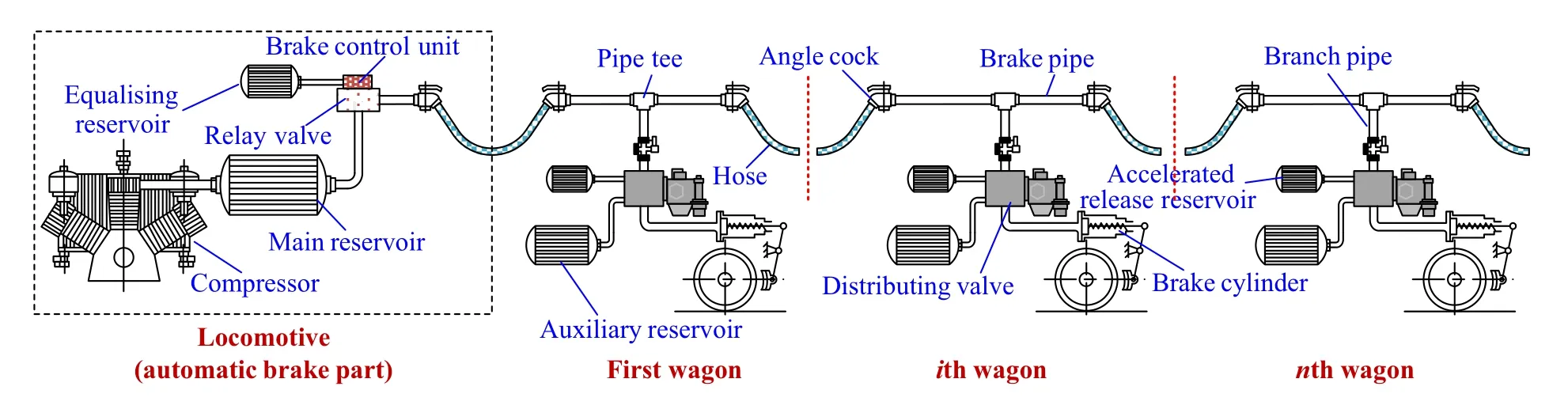
Fig.1 Train air brake system
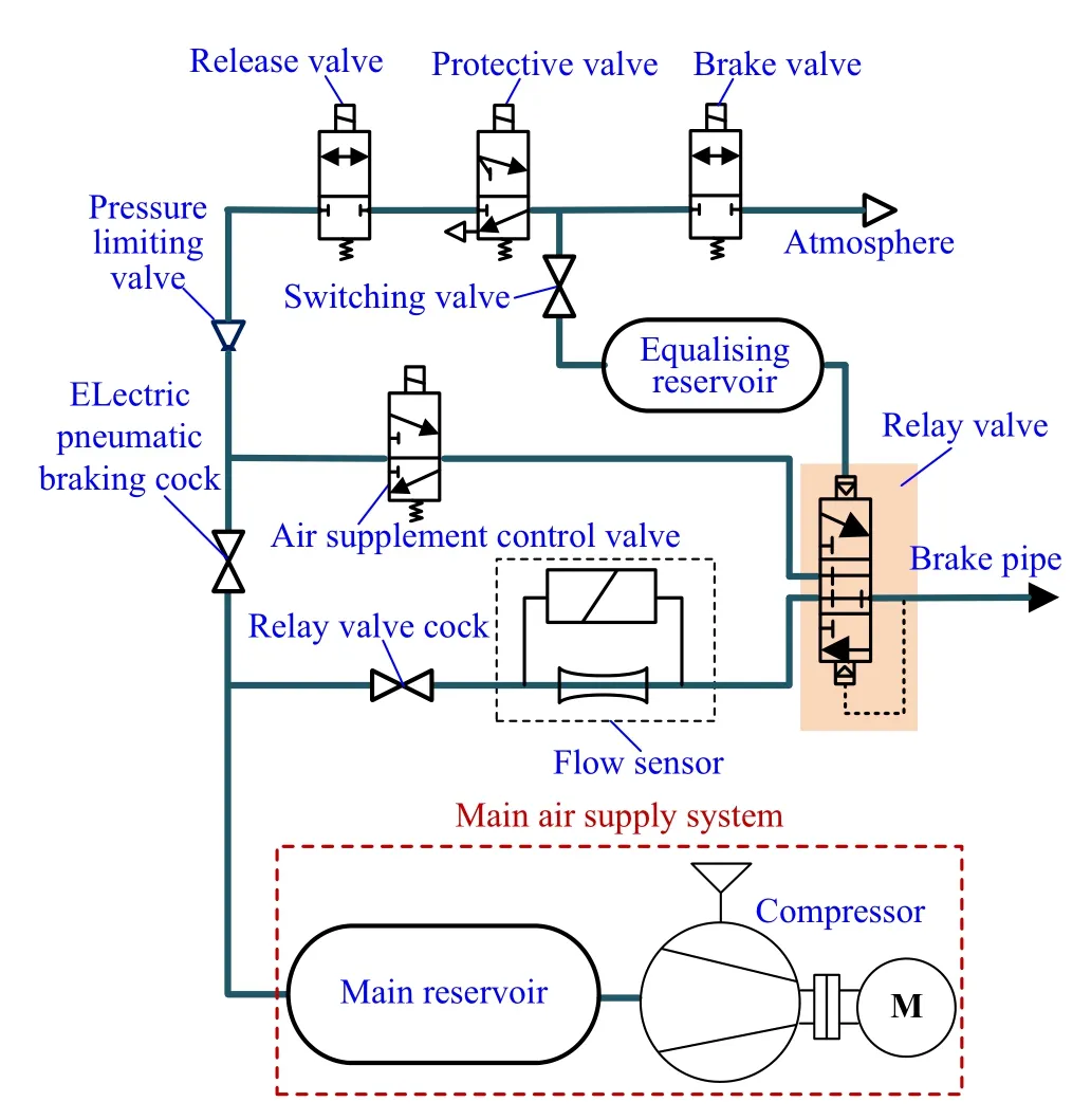
Fig.2 Schematic diagram of the typical electronically controlled pneumatic brake system of the locomotive
2.1 Locomotive brake system
Figure 2 shows the schematic diagram of a typical electronically controlled pneumatic brake system equipped for Chinese heavy-haul locomotives [31].It should be noted that only the automatic brake function of the locomotive is studied in this paper,and the independent brake function is not considered.The main air supply system,the basic part of the air brake system,is composed of the compressor and main reservoir (MR),which supplies pressurized air for the pneumatic parts and brakes of the locomotive and wagons.The system can automatically control the operation mode of the compressor according to the pressure signal of the MR,and thus the pressure of the MR can be maintained.When the automatic brake function is activated,the brake control unit receives commands from the automatic brake controller first,then the pressure of the equalizing reservoir (ER)is adjusted to the target value by controlling the opening and closing of the release and brake valves with pulse-width modulation (PWM) mode.The relay valve can regulate the pressure of the BP according to the ER pressure and the feedback BP pressure.
Apart from the above-mentioned parts,the system is equipped with other valves and cocks to accomplish the switch of braking modes,fault protection,etc.The pressure limiting valve can regulate the pressure of the pressurized air flowing into the ER from the MR.The relay valve cock and electric pneumatic braking cock control the on–offstates of connection paths of the MR to the relay valve and ER,respectively.The air supplement control valve can cut off the air supplement of the BP when the valve is closed.The switching valve can switch the braking mode from the electric pneumatic braking mode to the backup fully aircontrolled braking mode in fault conditions.Besides,the protective valve is equipped to discharge the ER when the power failure of the brake system occurs.
2.2 Wagon brake system
Each wagon is equipped with an independent air brake system which is connected to the BP through the branch pipe.The 120-type air brake is widely adopted by Chinese freight wagons,which is mainly composed of the main valve (MV),emergency valve (EV),semiautomatic release valve (SARV),pipe bracket,BC,auxiliary reservoir (AR),accelerated release reservoir (ARR),emergency chamber(EC),quick service bulb (QSB),etc.,as shown in Fig.3[32].The MV,the core part of the brake,consists of the main piston assembly (MPA),sliding valve (SV),graduating valve (GV),accelerated release valve (ARV),quick service valve (QSV),inshot valve,etc.The position of the MPA changes with the pressure difference between the upper and lower chambers,and the shoulder of the main piston stem further influences the positions of the SV and GV.It can be seen from Fig.4 that there are various ports,orifices,and connecting grooves in the GV,SV,and sliding valve seat (SVS),and different positions of the GV and SV form different air passages.Therefore,the brake can realize different service conditions in response to the change of the BP pressure.In this paper,the four common service conditions,namely the initial charging,release,service braking,and emergency braking,are studied.
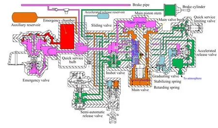
Fig.3 Schematic diagram of the 120-type air brake equipped for Chinese freight wagon (the release condition)
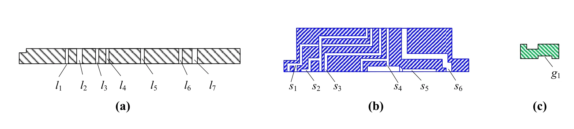
Fig.4 Ports,orifices,and connecting grooves on a the sliding valve seat,b the sliding valve,and c the graduating valve
(1)Initial charging.The MR charges the BP,and pressurized air flows into the upper chamber via the branch pipe and pipe bracket.The MPA moves down due to the pressure difference between the upper and lower chambers of the MV;meanwhile,the SV and the GV move down affected by the shoulder of the main piston stem till the SV contacts with the retarding spring seat.It can be seen from Fig.5a that the air passage between the BP and the lower chamber is formed via the upper chamber of the inshot valve,thel1on the SVS,and thes1on the SV;thus the AR can be charged.Besides,the pressurized air can flow into the ARR via thes2andl2.Another air passage links the BP and the lower chamber of the EV.The pressurized air flows into the EC via the axial hole,orifices III and IV of the emergency piston stem,and the backpressure of the vent valve is formed by charging the spring chamber.
(2)Release.The positions of the SV and GV under the release condition are the same as the initial charging condition,and the charging processes of the AR and EC are the same.As shown in Fig.3 and Fig.5a,pressurized air in the BC flows through the inshot valve,the SARV,thel1ands5on the SV and GV,the ARV,and finally to the atmosphere via orifice II.When the BC pressure is high,the piston stem of the ARV is laterally pushed to open the check valve,and the pressurized air in the ARR flows into the BP to accelerate the release process.When the ARR pressure is close to the BP pressure,the check valve of the ARV is closed.As the BP pressure increases to exceed the ARR pressure,the BP charges the ARR via the air passage in the MV similar to that of the initial charging process.When the pressure difference between the upper and lower chambers of the MV exceeds a certain value,the SV will push the retarding spring seat to move down,and the graduated charging position is achieved,as shown in Fig.5b.The upper orifice of the connecting grooves1is switched to connect to the orificel1.Because the upper orifice ofs1is narrower than the lower one,the charging rate of the AR is slowed down.
(3)Service braking.The BP pressure is reduced to the target value via the outlet vent of the relay valve in response to the service braking command.The upper chamber pressure of the MV decreases with the BP pressure,and the MPA moves up under the effect of the pressure difference between the upper and the lower chambers.The service braking process is divided into two stages.The first stage,namely the preliminary quick service,is that the GV moves up with the main piston stem about 6 mm,while the stabilizing spring force applied on the slide valve cannot overcome the static friction force between the SV and SVS,as shown in Fig.5c.Thel3,s3,g1,s4,andl5form an air passage that connects the BP and the QSB;meanwhile,the passage enables the BP to discharge to the atmosphere via orifice I.Thus the BP pressure is reduced quickly.In the second stage of the service braking,the increased pressure difference between the upper and lower chambers helps to overcome the friction force between the SV and SVS.Then,the MPA,the SV,and the GV further move to their top positions,as shown in Fig.5d.The connection between thel3ands3is cut off,and the preliminary quick service comes to the end.The BP starts to charge the BC through the air passage formed by thel5,s4,l4,the QSV,and the SARV.Besides,thes6andl7connect the lower chamber of the MV with the SARV;thus the pressurized air in AR can flow into the BC via this passage.When the BP pressure is reduced to the target value,the outlet vent of the relay valve is closed,while the AR still charges the BC in the initial few seconds.The pressure of the lower chamber continues to decrease;then the MPA and the GV move down under the effect of their gravity and the pressure difference until the upper shoulder of the MV stem contacts with the SV.It can be seen from Fig.5e that the two air passages to the BC in the second stage of the service braking are cut off,and a new air passage via thel1ands2is formed.The new air passage connects the BP with AR,which enables to keep the pressure difference at a small range.Therefore,the overcharge of the BC and the undesired release can be avoided.
(4)Emergency braking.During emergency braking,the movements of the parts in the MV are the same as those in service braking.Due to the rapid reduction of the BP pressure,the pressure difference between the upper and lower chambers of the EV promotes the down movement of the piston.Then,the pilot valve is opened,and the backpressure of the vent valve disappears,and the pilot valve push stem further pushes open the vent valve.Therefore,the BP can quickly discharge to the atmosphere,and the AR charges the BC (the first stage).With the decrease of the BP pressure and the increase of the BC pressure,the inshot valve piston is pushed to move up,and only the axial central hole of the piston stem stays open (the second stage).Then the charging rate of the AR is decelerated,which contributes to mitigating the longitudinal impulse of the train.
3 Mathematical model of the air brakes
As the electric logical control and the mechanical structures of the train air brake system are complicated,the system is simplified and described as a set of mathematical models.According to Figs.2,3,4 and 5,the system can be modeled as a series of reservoirs or chambers connected via pipes and orifices.Different service conditions are realized by opening or closing orifices in response to the control handle signal and the pressure change.The pressurized air is assumed to be an ideal gas,and all the transformations are isothermal.
3.1 Pipe model
The pipe is modeled as a constant-area one-dimensional duct,as shown in Fig.6.The pressurized air in the pipe is assumed to be isothermal,so the heat exchange between the air and pipe wall is omitted.Based on the conservations of mass and momentum,governing equations can be derived as

Fig.6 Control volume for the isothermal,constant area,frictional flow
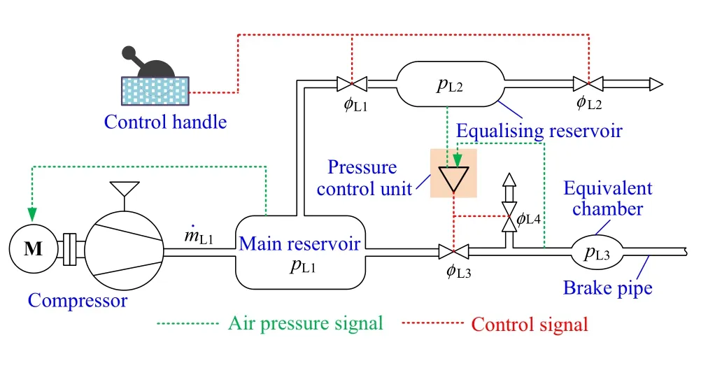
Fig.7 Equivalent model of the locomotive brake subsystem (automatic brake part)
whereρanduare the density and flow velocity of air,respectively;tis the time;zis the position along the pipe;pis the air pressure;dis the pipe diameter;nis the polytropic exponent of the ideal gas,andn=1 for isothermal assumption;fis the friction factor related to the pipe wall shear stressτw;Ris the gas constant;Tis the temperature.The pressure loss caused by connected components is considered as additional pipe wall friction by introducing the correction factorcfwhich can be expressed as
whereLandLeare the pipe length and equivalent length,respectively.More details about the equivalent length can be found in Ref.[17] and not presented here for brevity.
3.2 Modeling of locomotive brake system
Figure 7 shows the equivalent model of the locomotive brake subsystem (automatic brake part),which is mainly composed of the compressor,control handle,MR,ER,equivalent chamber,pressure control unit,and four orifices.The equivalent chamber is employed to deal with the boundary condition during numerical simulation,and more details will be introduced in the next section.The compressor is simplified as an air source that charges the MR with a certain mass flow according to the feedback MR pressure.The mass flow of the orifice () can be calculated using an empirical correlation as [18]
whereAdenotes the orifice area;CMis the Mach correction factor which can be calculated by
puandpddenote the inlet and outlet pressures,respectively;γdenotes the isentropic exponent;as the real flow is not necessarily isentropic due to the high irreversibility of the thermodynamic processes,an empirical correction factorCqby Perry is introduced:
Following mass conservation and neglecting kinetic energy,the pressure of the MR,ER,and equivalent chamber can be obtained by
whereVris the volume of the reservoir or the chamber;pris the pressure of the reservoir or the chamber;is the mass flow of theith orifice;djis the diameter of thejth pipe;ujis the air flow velocity of thejth pipe;NoandNpare numbers of orifices and pipes,respectively.It can be seen that the right side of Eq.(8) consists of two parts,namely the pressure change caused by the orifice flows and pipe flows,respectively.It should be noted that the inlet mass flow is defined to be positive,and the outlet mass flow is negative.As introduced in Sect.2.1,orificesϕL1andϕL2are controlled by the driver’s handle for regulating the ER pressure.The pressure control unit determines BP pressure by opening or closing the orificesϕL3andϕL4according to the ER pressure and feedback BP pressure.pL1,pL2,andpL3are pressures of the main reservoir,equalizing reservoir,and equivalent chamber,respectively.
3.3 Modeling of wagon brake system
The wagon air brake subsystem is connected to the BP via the branch pipe and pipe tee.The branch pipe model is the same as the BP model,and the pipe tee is modeled as boundary conditions (which will be presented later).According to Fig.8,the model is composed of the branch pipe,eight chambers or reservoirs (pw1,pw2,…,pw8),thirteen orifices(ϕw1,ϕw2,…,ϕw13),MPA,etc.The equivalent chamber is introduced to model the connection area to the branch pipe,emergency valve,and upper chamber of the main valve.
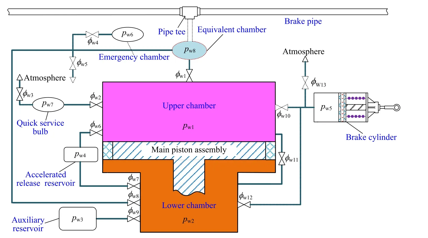
Fig.8 Equivalent model of the wagon air brake subsystem
As introduced in Sect.2.2,the pressure change of the BP affects the movement of pistons of the MV and EV.The positions of SV and GV change with the MPA,and different air passages are formed to connect different chambers or reservoirs.According to the structures of the MV,the equations of motion of the MPA,GV,and SV can be obtained.The initial positions of all moving parts are defined as in Fig.5a,where the displacements of the MPA (xp),GV,and SV (xs)are zero,and the relative displacement between the MPA and SV (xps) is zero either.Besides,the upward movement is defined as positive.To determine the motions of moving parts,the dynamic forces and friction forces should be compared first.As the MPA and GV always move together,the two parts are treated as a whole.The friction force applied on the SV (Fs) is larger than the maximum stabilizing spring force;thus the SV can move only when the upper or lower shoulder of the piston stem contacts with it.According to the relative position between the MPA and SV,the equations of motion are classified into three conditions.
Condition 1xps=0,as shown in Fig.5a,b,and e.The upper shoulder of the piston stem contacts with the SV,and the stabilizing spring is not deflected relative to the initial position.Under the effect of the piston force (Fp) caused by the pressure difference between upper and lower chambers,the MPA will keep still,or move down with the SV,or move up while the SV stays still.The equations of motion under different force and displacement conditions are expressed as
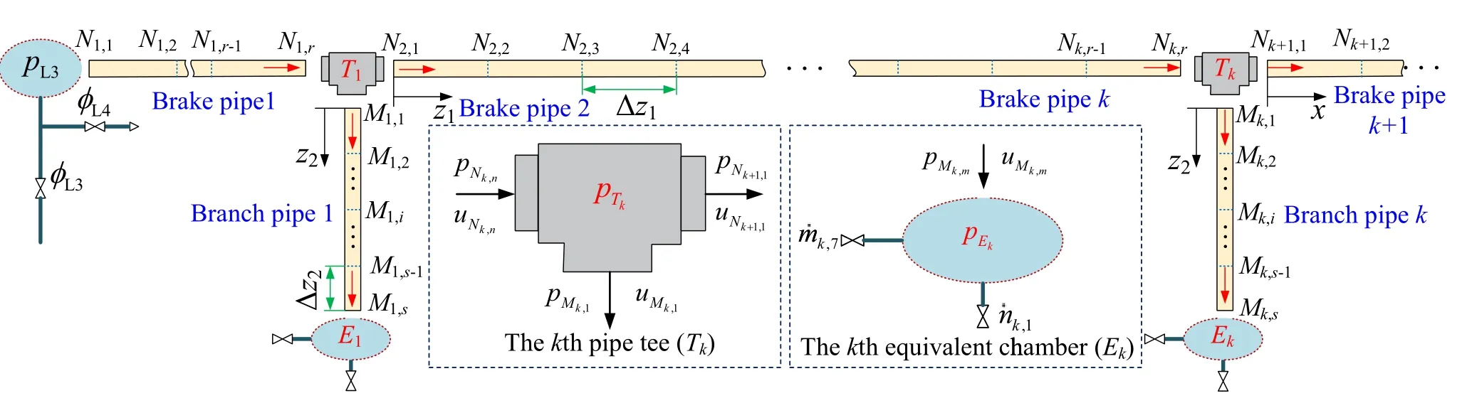
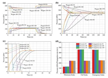
Condition 2 0 Condition 3xps=xpsmax.The lower shoulder of the piston stem contacts with the SV.Similar to that under condition 1,the MPA and GV can stay still,or move up with the SV,or move down while the SV keeps still. Based on Eqs.(9)–(11),the acceleration of the MPA can be determined,and its velocity and displacement can be further calculated.According to thexpandxps,the position of the SV can be obtained as wherexs0is the displacement of the SV in the previous time step.As the positions of the SV,GV,and MPA have been calculated,the air passages can be determined according to Fig.5a–e.Therefore,different service conditions of the brake can be realized by controlling the opening sizes of orificesϕw1–ϕw13according to the positions of the GV and SV illustrated in Sect.2.2. The mass flows of orifices can be determined according to Eqs.(5)–(7).The EV is simplified as two orifices that are connected to the ER (ϕw4) and atmosphere (ϕw5),respectively.Theϕw5is opened only when the pressure difference between the ER (pw6) and equivalent chamber(pw8) attains the critical value.For chambers or reservoirs excepting the brake cylinder,their pressure can be calculated according to Eq.(8).The volume change of upper and lower chambers caused by the movement of the MPA is not considered herein.The BC is modeled as a chamber with variable volume,and it is assumed that there is no flow through the piston,as shown in Fig.9.The movement of the BC piston can be expressed as Fig.9 Brake cylinder model wheremb,cb,andkrdenote the mass of the BC piston,viscous friction constant,and the release spring stiffness,respectively;andybare the acceleration,velocity,and displacement of the piston,respectively;Abis the transversal area of the piston;pw5andpatmare BC pressure and atmospheric pressure,respectively;Fpreis the preload of the release spring.The BC pressure considering the variable volume with time is described by wherey0is the equivalent piston displacement of the dead volume;is the sum of mass flow into the BC. The air brake subsystems of the locomotives and wagons are connected by brake pipes,branch pipes,and pipe tees.To simulate the train air brake system,the subsystems should be integrated through boundary conditions,as shown in Fig.10.In the Figure,Nk,iandMk,jdenote node numbers of brake pipes and branch pipes,respectively;the subscriptkdenotes the pipe number,and subscriptsi(i=1,2,…,r) andj(j=1,2,…,s) denote node numbers in each brake pipe and branch pipe,respectively;here,therandsare the total number of nodes for each brake pipe and branch pipe,respectively,which are determined by the mesh sizes.The air flow in the pipe is described by Eqs.(1)–(4) and is solved using the finite-difference method.Taking thekth brake pipe as an example,the difference scheme,a backward approach in Eq.(1) and a forward approach in Eq.(2),is expressed as Fig.10 Integration of the train air brake system model The pipe tees (T1,T2,…,Tk) and equivalent chambers (E1,E2,…,Ek) are modeled as small chambers with fixed volume,and the pressures of pipe nodes connected to the pipe tees or equivalent chambers are assumed to be equal [13].For the first node of a pipe,the node pressure equals the pressure of the chamber.As the flow velocity of the first node can be obtained by Eq.(15),the chamber pressure can be calculated according to Eq.(8).For the last node of a pipe,the flow velocity can be obtained by equating the derivative of pressure as givenby Eqs.(8) and (15).The boundary conditions are given as follows: The close end: The brake pipe: The branch pipe: In above formulations,VTandVEare volumes of the pipe tee and the equivalent chamber of the wagon brake model,respectively;d1andd2are diameters of the brake pipe and branch pipe,respectively;are pressures of nodeMk,sandMk,s−1,respectively;are air flow velocities of nodeMk,sandMk,s−1,respectively;is the mass flow of orificeϕw1in thekth wagon brake;is the total mass flow of orificesϕw4,ϕw5andϕw8in thekth wagon brake.The modeling of the train air brake system and the boundary conditions are described by Eqs.(1)–(18),and the dynamic characteristics of the system can be calculated by numerical integrations. When solving Eq.(15),it is recommended to determine the pressure first and then calculate the air flow velocity with new pressure rather than the pressure at the previous integration step.According to the author’s numerical experiments,this little change in programming can significantly improve algorithm stability.Compared with the commonly used method of characteristics with the consideration of energy,the proposed method in this paper can avoid iterations when calculating pipe boundary conditions;thus the model can achieve high computational efficiency. Based on the above-introduced method,a simulation model that consists of 150 sets of wagon air brake systems was developed by in-house code using MATLAB.Key parameters of the brake system were set according to Ref.[28].The operating pressure was set to be 600 kPa,which is the norm in Chinese heavy-haul railway.Note that all the pressures in simulation results presented in this paper are gauge pressures.The mesh sizes of brake pipes and branch pipes were 0.96 and 0.75 m,respectively.Through a large number of numerical experiments,the maximum time step that can reflect the details of push rod extensions during the service and emergency braking is about 0.2 ms.In the following simulations,the time step is set to be 0.2 ms.Figure 11a–c presents the BP and BC pressures of the first wagon (001),the middle wagon (075),and the last wagon (150) under conditions with different pressure reductions in the brake pipe,respectively. It can be seen from Fig.11a that the BP pressure of the first wagon is rapidly reduced to the target pressure,while the BP pressures of the middle and last wagons decrease slowly after the quick service and attain the target pressure at aboutt=60 s.Reductions of BP pressures lead to the movement of the MV,GV,and SV,and then the AR charges the BC;meanwhile,the BP charges the BC at the second stage of quick service.With the increase of the BC pressures,the BC piston rods are extended after the preload of the BC release spring is overcome,and the ascending rate of the BC pressure is slowed down during the extending of the piston rod.For the middle and last wagons,the stagnations of BC pressures can be observed during brake application.This phenomenon is caused by the fluctuation of the pressure difference between the upper and lower chambers of the MV.The fluctuating pressure difference makes the service condition of the wagon air brake switch between the brake and lapping.The brake release operation is applied att=100 s,and an abrupt pressure increase of the BP quick release can be seen in the initial stage of the release.Unlike the brake operation,the BC pressure curves of different wagons during brake release are uniform.The decrease rate of the BC pressure is slowed down during the retracting of the piston rod. Similar to the minimum brake condition,the BP pressure descending rate and BC pressure ascending rate of the first wagon are larger than those of the middle and last wagons under the full brake condition with a 170 kPa pressure reduction in the BP,as shown in Fig.11b.As the BP pressure reduction of full brake is larger compared to the minimum brake condition,the duration of the BP depressurization and BC pressurization are longer,accordingly,the BC pressure is higher.Besides,the stagnation of BC pressures can be observed in the middle and last wagons.At aboutt=118 s,the BC pressure of the last wagon attains the maximum value(about 455 kPa).For the emergency brake condition,the BP and BC pressure curves of different wagons are uniform.The BP pressures are reduced to 0 kPa within 10 s,and the BC pressure of the last wagon reaches its maximum value at aboutt=18 s.It can be seen that the BC pressures increase rapidly to about 150 kPa during the first stage of the emergency brake,and then the pressure ascending rate is reduced due to the decreased opening size of air passage between the AR and BC caused by the movement of the inshot valve.The maximum BC pressure of emergency brake condition nearly equals that of the full brake condition,and the stagnations of BC pressures do not occur.Figure 11d shows comparisons of the simulated average maximum cylinder pressures and brake application propagation rates with the measured data in Ref.[28].It can be seen that the simulated average pressures and propagation rates under different service conditions are close to the measured data.Besides,the pressure curves in Fig.11a–c are consistent with the measured data in Ref.[28] as well.Therefore,the developed simulation model can rationally simulate the characteristics of the air brake system. Focusing on the commonly used train formations in Chinese heavy-haul railways,we further studied the air brake characteristics of trains with different sets of wagons.The 5000-t level and 10,000-t level trains are generally composed of 54 and 108 wagons,respectively.The BP and BC pressure curves of the first and last wagons of three train formations for different service conditions are displayed in Fig.12a–c.Both the BP and BC pressure curves of the first wagon are close under different train formations while the pressure curves of the last wagon differ a lot.For the emergency brake condition,the main difference in air brake characteristics for the three train formations lies in the time delay caused by the brake pipe length.For the minimum and full brake conditions,the stagnation phenomenon of BC pressures is more significant in a longer marshaling apart from the time delay.The larger the train formation is,the longer the duration of the BP depressurization and BC pressurization are.As shown in Fig.12d,the average maximum cylinder pressures and brake application propagation rates are close for different train formations.In the longitudinal train dynamics simulation,the empirical air brake model originating from the measured data of a certain train formation can only be rationally extended to simulate the emergency brake behavior of other train formations.For service braking conditions with different pressure reductions in the brake pipe,the test facilities or fluid dynamics models are recommended to acquire accurate air brake characteristics of a certain train formation. Fig.12 Simulation results of models with different sets of wagon air brake systems a minimum brake of 50 kPa reduction,b full brake of 170 kPa reduction,c emergency braking,d average maximum cylinder pressures and brake application propagation rates This paper has proposed an approach for modeling and solving the air brake system based on fluid dynamics theory.The mathematical models of locomotive and wagon air brake systems considering the air flow in the brake pipes and branch pipes and dynamic motions of valves are established according to their structures and working mechanisms.The simulation model of the whole air brake system is developed,and the solving method utilizing the finite-difference method is illustrated.Besides,new efficient pipe boundary conditions without iterations are developed,which can achieve high computational efficiency.The developed model was validated using the published measured data in the literature.The simulation results of different train formations indicate that the dynamic behavior of brake pipes is more likely to cause stagnations of brake cylinder pressures in the rear wagons of a long train during service braking.The fluid dynamics model is better for predicting the characteristics of long trains under service braking conditions while the simple empirical models considering the time delay and measured brake cylinder pressures can meet the demand of emergency braking simulations. AcknowledgementsThis work was supported by the National Natural Science Foundation of China (Grant Nos.51825504,51735012,and 52072317).The authors would like to thank the State Key Laboratory of Traction Power for providing equipment and materials for this project,and also acknowledge the Xplorer Prize for sponsoring the project. Open AccessThis article is licensed under a Creative Commons Attribution 4.0 International License,which permits use,sharing,adaptation,distribution and reproduction in any medium or format,as long as you give appropriate credit to the original author(s) and the source,provide a link to the Creative Commons licence,and indicate if changes were made.The images or other third party material in this article are included in the article’s Creative Commons licence,unless indicated otherwise in a credit line to the material.If material is not included in the article’s Creative Commons licence and your intended use is not permitted by statutory regulation or exceeds the permitted use,you will need to obtain permission directly from the copyright holder.To view a copy of this licence,visit http:// creat iveco mmons.org/ licen ses/ by/4.0/.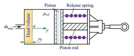
4 Numerical formulations of the air brake system
5 Simulation and discussion
6 Conclusion
杂志排行

Railway Engineering Science的其它文章
- The effect of controllable train-tail devices on the longitudinal impulse of the combined trains under initial braking
- A numerical method for the simulation of freight train emergency braking operations based on the UIC braked weight percentage
- Influence of quick release valve on braking performance and coupler force of heavy haul train
- A simplified pneumatic model for air brake of passenger trains
- Braking distance prediction for vehicle consist in low-speed on-sight operation: a Monte Carlo approach
- HIL testing of wheel slide protection systems: criteria for continuous updating and validation