Comparative analysis on gas-solid drag models in MFIX-DEM simulations of bubbling fluidized bed
2023-02-28RuiyuLiXiaoleHuangYuhaoWuLingxiaoDongSrdjanBeloeviAleksandarMilieviIvanTomanoviLeiDengDefuChe
Ruiyu Li, Xiaole Huang, Yuhao Wu, Lingxiao Dong, Srdjan Belošević , Aleksandar Milićević ,Ivan Tomanović , Lei Deng,, Defu Che
1 State Key Laboratory of Multiphase Flow in Power Engineering, School of Energy and Power Engineering, Xi’an Jiaotong University, Xi’an 710049, China
2 Shunde Institute of Inspection, Guangdong Institute of Special Equipment Inspection and Research, Foshan 528300, China 3 Department of Thermal Engineering and Energy, ‘‘VINČA‘‘ Institute of Nuclear Sciences - National Institute of the Republic of Serbia, University of Belgrade, Mike Petrovića Alasa 12-14, 11351 Vinča, PO Box 522, 11001 Belgrade, Serbia
Keywords:MFIX-DEM Simulation Dense flow Gas-solid Bubbling fluidized bed Drag model
ABSTRACT In this study, the open-source software MFIX-DEM simulations of a bubbling fluidized bed (BFB) are applied to assess nine drag models according to experimental and direct numerical simulation (DNS)results.The influence of superficial gas velocity on gas-solid flow is also examined.The results show that according to the distribution of time-averaged particle axial velocity in y direction, except for Wen-Yu and Tenneti-Garg-Subramaniam (TGS), other drag models are consistent with the experimental and DNS results.For the TGS drag model, the layer-by-layer movement of particles is observed, which indicates the particle velocity is not correctly predicted.The time domain and frequency domain analysis results of pressure drop of each drag model are similar.It is recommended to use the drag model derived from DNS or fine grid computational fluid dynamics-discrete element method (CFD-DEM) data first for CFD-DEM simulations.For the investigated BFB, the superficial gas velocity less than 0.9 m·s-1 should be adopted to obtain normal hydrodynamics.
1.Introduction
Bubbling fluidized bed has been extensively employed in industry for decades,because of its high heat transfer rate and well gassolid contact [1].It is significant to investigate hydrodynamics to ensure the normal operation of bubbling fluidized bed (BFB) [2].Some flow characteristics, such as pressure drop, bed height, and voidage profile, are available from experimental studies [3-5].But due to the large number of particles and limited detection technologies,it is difficult to obtain the detailed particle-scale data from experiments for the in-depth study.
Recently, computational fluid dynamics (CFD) becomes a conspicuous tool to study hydrodynamics at a particle-scale.CFD methods mainly include particle-resolved direct numerical simulation (PR-DNS) [6,7], computational fluid dynamics-discrete element method (CFD-DEM) [8,9], multi-phase particle-in-cell (MPPIC) [10,11], and two-fluid method (TFM) [12,13].Among them,CFD-DEM can get data at a particle-scale without consuming too many resources.At the same time, this method is much easier to consider the effect of forces on particles by modifying the CFD code.Thus, CFD-DEM is extensively applied in particle-scale studies [14-16].
For the common fluidized bed,it is considered that particles are subjected to drag force, lift force, pressure gradient force, gravity,and collisions [17].On the basis of Lu et al.[2] and Wang [17],the drag force is the predominant of all the forces.In CFD-DEM studies, the drag force can be calculated by empirical correlations,which could be derived (1) from experimental data [18,19], (2) by assuming the force balance of a single particle [20], (3) through hybrid drag models[21],(4)from DNS data[22,23],(5)from highly resolved TFM or CFD-DEM results [1,24,25], and (6) via energy minimization multiscale(EMMS)drag models[26,27].Many studies have been reported to assess the performance of different drag models in fluidized beds [1,8,9,11,28-48].However, only a few CFD-DEM studies have been conducted [8,9,29-32,39,40,49].In addition, according to Agrawal et al.[49], the performance of drag models would vary at different superficial gas velocities (Ug).Unfortunately, among these limited CFD-DEM studies, only a few studies have focused on the effect of small-scale Ugchanges on gas-solid flow [8,9,28].Moreover, new drag models proposed in recent years [1,24] are lacking of validation.To our knowledge,for the above two drag models, only three studies have been conducted to verify them [1,50,51], while two of them are conducted by the model proposers themselves.These new drag models urgently need to be validated against classic drag models.
In this study,nine drag models are evaluated based on the previous experiments[52]and DNS study[7].To balance accuracy and computing efficiency, CFD-DEM is adopted.Simulations are based on an open-source software MFIX-DEM (version 21.1.4), which is developed by National Energy Technology Laboratory (NETL) and has been proven to provide convincing results of fluidized bed simulations[53-56].First,the cases are verified based on the flow pattern and velocity profile.Then, time-averaged and instantaneous characteristics, including pressure drop, voidage, angular velocity,granular temperature, and interphase energy transfer rate are compared.At last, the influence of Ugon gas-solid flow is examined.This comparative analysis could provide an important reference for the selection of drag models for BFBs.
2.Numerical Simulation
2.1.Governing equations and interphase drag model
In MFIX-DEM [57], for particle i (i = 1, 2, ···, N), the particle motion is represented in the Lagrangian frame at time t withparameterswheredenotes particle diameter,represents particle mass,expresses particle density,X(i)(t)denotes particle position,(t)represents particle linear velocity,and ω(i)(t) expresses particle angular velocity.In the current study, it is assumed that both the diameter and the density of particles are constant, indicating thatandare replaced by dpand ρs,respectively.The above parameters are given as follows:
where g is the acceleration due to gravity,Fdis the total drag force(pressure plus viscous) on the ithparticle residing in kthcell and belonging to the solid phase, Fcis the net contact force acting as a result of contact with other particles, and T(i)is the sum of all torques acting on the ithparticle [58].
Meanwhile, the gas phase governing equations are implemented as follows:
where βDEMis related to gas-solid interphase drag coefficient β:
The drag coefficient β is calculated from nine correlations summarized in Table 1, depending on the model.For convenience,abbreviations of all models are given in parentheses.In MFIXDEM,the implicitness calculation code of the gas-solids drag coefficient is stored in drag_gs.f and drag_gp_des.f.If the code of drag model is modified,the input and output parameters of the subroutine in the above two files must be consistent.With respect to Table 1,please note that(1)due to the different definitions of Reynolds number,the Syamal drag model here has been rewritten for convenient reading, and (2) EMMS models are not considered in the current study.Although EMMS models have been successfully applied in TFM[60-63],its performance in CFD-DEM remains to be observed, which is outside the range of this study.
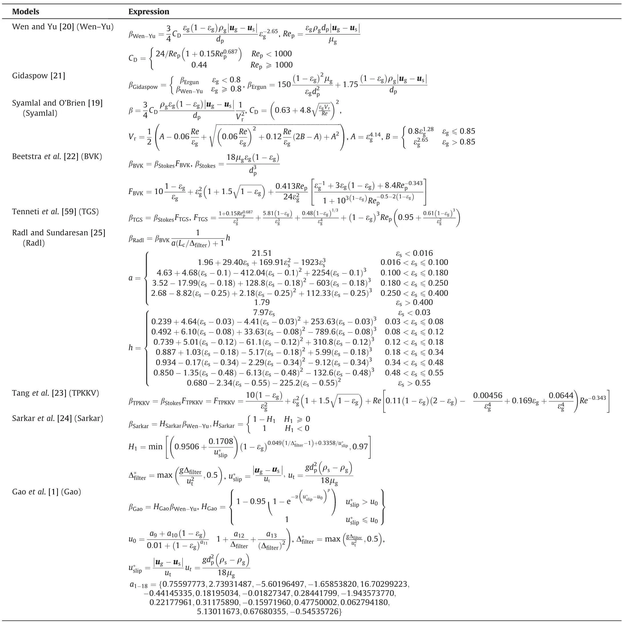
Table 1 Summary of drag model correlations
2.2.Collision model
From Eq.(2), the contact force is vital to correctly capture the motion of particle.In this study, a linear spring-dashpot (LSD)model, namely soft-sphere model [64] is employed to calculate the contact force, which is broken down into a normal one (Fn)and a tangential one (Ft).These two components are expressed as the following [8]:
where αsis the friction coefficient, k is the spring constant, δ is the overlap between particles,η is the damping factors,and subscript n,t,r stands for normal,tangential,relative velocity,respectively.LSD model performs better than the hard-sphere model (e.g.Hertzian model) [65] in the dense gas-solid flow, because its time step is independent of the voidage [58].Regarding the influence of the choice of collision model, a recent research can be referred [8].
2.3.Particle granular temperature
In a dense gas-solid system,the relative movement among particles affects the drag force.To characterize the fluctuation of particle velocity, the particle granular temperature θ is implemented as the following:
where i is the direction x,y,or z,us,ik(x,t )is the instantaneous velocity of the kthparticle in i direction, n is the particle number in the cell,and ci(x,t ) is the mean velocity in i direction in the cell,which is defined by the following:
2.4.Numerical setting
With reference to the DNS [7] and experimental studies [52], a fluidized bed of dimensions 44 mm×133.2 mm×10 mm is established,as shown in Fig.1.According to Luo et al.[7],the minimum fluidization velocity(umf)of current fluidized bed is 0.3 m·s-1.The particle size is 1.2 mm.It is a mono-sized particle system.The cell numbers are 12 × 24 × 3.The minimum cell size is around 3dp,which is considered to be appropriate [25,66].At the initial moment,9240 particles are regularly arranged in the fluidized bed.The initial bed height is 39.6 mm(33dp).The air enters evenly from the bottom surface,then flows out from the upper surface,which is set as a pressure outlet condition with 1.0132 × 10⁵Pa.The nonslip wall boundary condition is applied to other walls.Detailed parameters are given in Supplementary Material.Note that the normal restitution coefficient adopts the setting in Luo et al.[7]for comparison with PR-DNS data.It explains why the normal restitution coefficient in this study is uncommon.Furthermore,each case is calculated for 30.0 s.In the following,unless otherwise indicated, the last 20.0 s of data is used to ensure stable flow.

Fig.1.Schematic of simulation domain.
3.Results and Discussion
3.1.Model validation
In this section,the axial velocity distribution are present for validation.Fig.2 represents time-averaged particle axial velocities in y direction uywith the Ugof 0.9 m·s-1using different drag models,compared with the experimental[52]and DNS[7]data.Except for TGS,the models predict that particles in the center move upwards,and the near walls move downwards, which is a typical particle circulation method in BFBs and has received wide coverage[1,9,49].Besides,at y=15 mm,CFD-DEM results are close to experimental and DNS results.As the height increases, the deviation becomes larger.At y = 25 mm and y = 35 mm sections, uyof CFD-DEM near the wall and the center is obviously lower than that of experiment and DNS.The similar situation is also reported by Bian et al.[9].This could be attributed to two reasons.First, the current drag models tend to underestimate the drag force[9,30,67-70], resulting in a lower time-averaged section velocity.Second,the error of velocity is also caused by the effect of the wall and coarse mesh [8].The advanced fine-grid CFD-DEM method considering the boundary layer is in urgent need [71], but beyond the scope of this study.Furthermore, TGS and, to some degree,Wen-Yu behaves unusually compared with the others.The typical circulation method mentioned above is unapparent when using Wen-Yu drag model.Especially at y = 35 mm, the difference of uybetween the wall and center is significantly smaller.For TGS,uyis almost constant along x direction at all sections.To summarize, the current MFIX-DEM simulation could capture the characteristics of particle motion in the BFB.The validation results are acceptable to some extent.
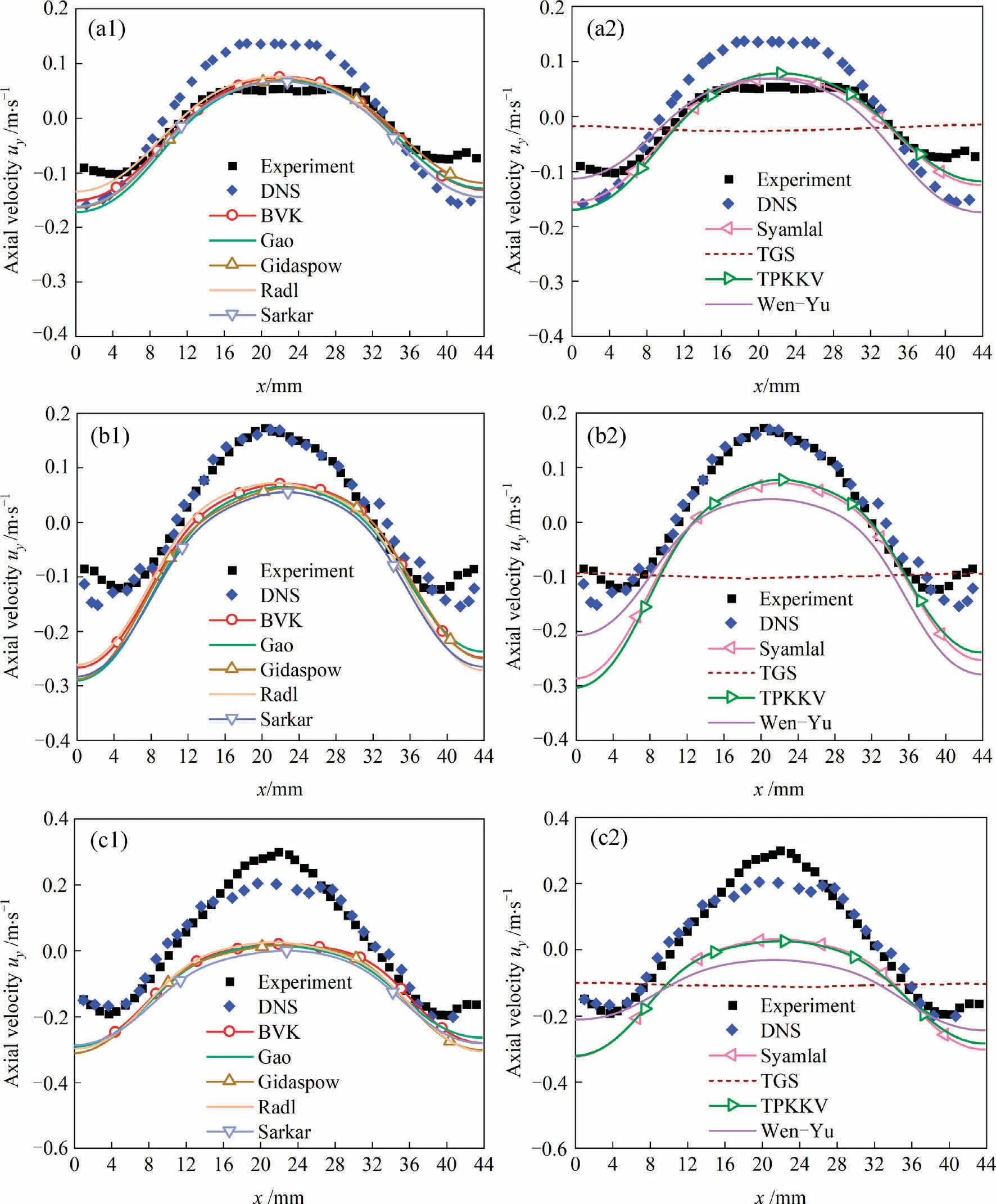
Fig.2.Time-averaged particle axial velocity in y direction compared with experimental and DNS study at: (a1, a2) 15 mm, (b1, b2) 25 mm, and (c1, c2) 35 mm heights sections.
3.2.Comparison of different drag models
3.2.1.Pressure drop
The pressure drop is an important quantity to measure the operation of the fluidized bed.For BFBs, unusual pressure drops often indicate operational problems,such as particle escape or fluidization failure.In this section, the pressure drop is expressed as the averaged pressure at the bottom plane (y = 0.5h) minus that at the top plane(y=H-0.5h)[30,72],where h is the calculation cell size in y direction:
To investigate the characteristics of pressure drops, the frequency domain analysis is adopted in this study.Through Fourier transform, the time domain signal of pressure drop from Eq.(12)can be converted into frequency domain signal, as shown in Fig.SM-1(in Supplementary Material).The power variation trends of MSA with frequency are the same.For all drag models,the main frequencies can be easily found in the low frequency region.The main frequency of Wen-Yu is the highest (3.797 Hz), while the lowest is Gidaspow(3.198 Hz).In general, there is little difference between the main frequencies of nine drag models.
The time-averaged pressure drop with the Ugof 0.9 m·s-1is applied in Fig.3.The last 20.0 s of data are used for plotting.Results of all drag models are pretty close,around 150.0 Pa.From time and frequency domain analysis,it demonstrates that the pressure drop is not sensitive to the selection of drag model, especially for the time-averaged results.The similar conclusion could be found in the study of Bian et al.[30].
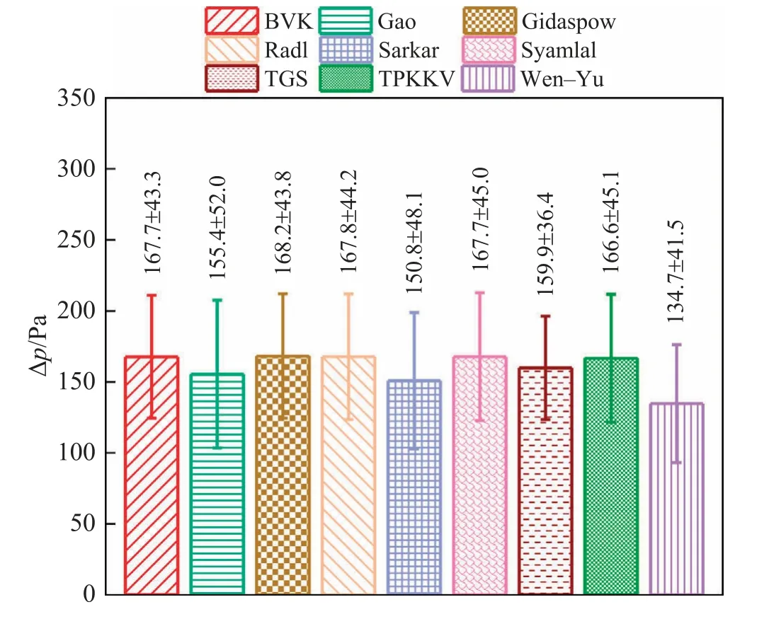
Fig.3.Time-averaged pressure drop using different drag models.
3.2.2.Voidage
In this section, for further discussion, voidage profile is divided into two parts,including instantaneous and time-averaged results.Fig.4 represents the voidage profile at 15.0 s with the Ugof 0.9 m·s-1.A series of bubble appears, including the bubble‘‘formation-rising-breaking-fall‘‘, observable from Fig.4 at the same time.That is to say, the instantaneous results of different drag models are significantly different.Note that TGS has a distinctive performance.At different heights, the voidage of TGS along x direction is almost constant, similar to the distribution of uy.Fig.SM-2 represents the time-averaged voidage profile with the Ugof 0.9 m·s-1.Obviously, the voidage simulated by TGS model is almost constant along the x direction.Combined with Figs.2,4, and SM-2, it is concluded that the particles move ‘‘layer-bylayer” when using TGS drag model in the investigated BFB.To our knowledge, this curious phenomenon has not been reported yet,although TGS drag model has been used in many researches[54,73-76].A possible explanation is that the TGS model is suitable for the range of voidage from 0.5 to 0.9 [63], resulting in an unrealistic gas-solid flow simulation.Another reason could be that the TGS drag model is too small to fully fluidize the particles.The system is actually operated at the one-dimensional travelling wave stage.

Fig.4.Instantaneous voidage profile of the BFB at 15.0 s.
3.2.3.Angular velocity
The time-averaged angular velocities in y direction ωyat three heights are shown in Fig.5.Other than the particle axial velocity,the angular velocity is irregularly distributed along x direction.The curve of TGS fluctuates irregularly, like in the case of other models.
The similar situation is discovered in Fig.SM-3, where the section-averaged ωyat the three heights is represented.There is no rule that could effectively explain the results of all models in Figs.5 and SM-3.No drag force model has special performance.Wang et al.[8]considered that the rotation of particles in the upper part (y = 20 mm) was stronger than that in the lower part(y = 10 mm).However, this phenomenon is not observed in this study.From Fig.SM-3, for BVK and Radl, the ωyat y = 35 mm is the highest.For Gao, Gidaspow, Sarkar, TGS, and TPKKV, the ωyat y = 25 mm is the biggest.For Syamlal and Wen-Yu, the ωyat y=15 mm is the highest.A unified conclusion could not be drawn on where the rotation intensity is the strongest in the investigated BFB.
In addition, the influence of angular velocity on the performance of drag model has not been fully discussed by researchers.Sun and Battaglia[77]proposed an improved Eulerian model combined with particle rotation, which is closer to the experimental data.Considering the influence of particle rotation could be a direction to further improve drag models.
3.2.4.Granular temperature
Fig.6 shows the time-averaged results of particle granular temperature in y direction θyyat 15, 25 and 35 mm heights sections with the Ugof 0.9 m·s-1.Except for the TGS and Wen-Yu,the maximum of granular temperature appears around x = 6 mm and x = 38 mm while the minimum appears around x = 22 mm, distributed in an ‘‘M‘‘ shape.

Fig.6.Time-averaged granular temperature in y direction θyy at: (a1, a2) 15 mm, (b1, b2) 25 mm, and (c1, c2) 35 mm heights sections.
The similar granular temperature distribution was mentioned in previous studies [8,52].It could be inferred that affected by the particle circulation, the particle number in the center tends to be small, leading to fewer particle-particle collisions.Thus,the velocity difference among particles is limited, resulting in a small granular temperature in the center of investigated BFB.Different from the case near the central axis, the slight decrease of granular temperature around the wall is observed attributed to the impact of wall and the falling process in the particle circulation.At y = 15 mm, the Wen-Yu drag model performs the same as others.However, as the height rises, the central granular temperature is gradually higher than other models, while the peaks near the wall gradually decrease.When y = 35 mm,the two peaks around x = 6 mm and x = 38 mm almost disappear.For TGS, the granular temperature along x direction is almost unchanged,which is similar with the particle axial velocity distribution in Fig.2.It demonstrates that the particle velocity could not be well estimated by TGS and Wen-Yu.According to Eqs.(9), (10) and (11), the particle velocity determines the granular temperature.Therefore, it is inferred that the incorrect prediction of the particle velocity is the reason for the individual profile of granular temperature.
The global granular temperature (GGT) is adopted to stand for the global fluctuations of particle velocity, which is the average of all particles’ granular temperatures.The time-averaged results of GGT and granular temperature at three heights are reported in Fig.7.The value of TGS in the graph is always the lowest.Except for y = 15 mm, the value of Wen-Yu is the second lowest, which corresponds to the previous discussion in this section.It further proves that Wen-Yu and TGS are not suitable for the investigated BFB.Furthermore,it can be observed that the values of GGT for the three models are all on the order of 10-3,whereas θ is on the order of 10-2.In fact,the y=15 mm,y=25 mm and y=35 mm sections discussed in this section are all in the dense regime,which belongs to the region with large velocity fluctuations and large θ.Taken as a whole, it is reasonable that GGT is an order of magnitude smaller than θ.
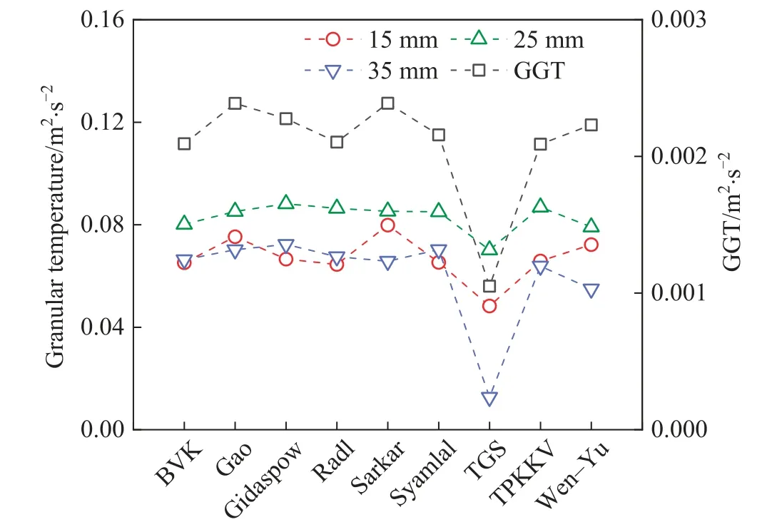
Fig.7.Global granular temperature (GGT) and granular temperature at 15 mm,25 mm, and 35 mm heights sections using different drag models.
3.2.5.Interphase energy transfer rate
The change of interphase energy transfer rate over time is summarized in Fig.SM-4.In BFBs, the energy obtained by the particle group is converted into kinetic energy, part of which is dissipated in collision and friction.All the above energies are provided by the gas.Therefore, understanding the gas-solid energy transfer process is of crucial significant to correctly describe the particle motion.In CFD-DEM,the interphase energy transfer rate is formulated as follows [9]:
where Npand Vpare the particle number and particle volume, usiand ugiare the interpolation of solid and gas velocity at the center of ithparticle, respectively.
Note that: (1) in the MFIX code, the function f_gp(i) stands for the particle-centred drag coefficient for ithparticle, which equals to the βDEMin Eq.(6);(2)Fig.SM-4(a)is drawn using WebPlotDigitizer(https://apps.automeris.io/wpd/index.zh_CN.html)to extract data points based on the graph in the study[7];(3)due to the limited data given in the experimental and DNS study,the interphase energy transfer rate is the only parameter that can be directly compared with the literature; (4) restricted by computing resources,Luo et al.[7] simulated 2.7 s, of which 1.8 s were displayed in Fig.SM-4(a).To make it easier to see the image, only the data in the current work of 0-7.0 s is statistically plotted in Fig.SM-4(b)to SM-4(j).
At first, CFD-DEM results are wildly different from DNS results due to various initial conditions.After that, all the power curves oscillate around zero, but the amplitude of CFD-DEM is significantly larger than that of DNS.In Fig.SM-4,once again,the fluctuation of TGS drag model is small and exceptionally regular,like the pressure drop curve shown in Fig.SM-1(g).Detailed mean and standard deviations of interphase energy transfer rate are given in Fig.8.
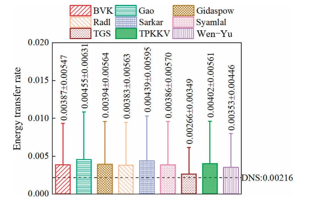
Fig.8.Time-averaged interphase energy transfer rates using different drag models.
Apparently,the results from all models are greater than that of DNS study.TGS has the closest result to DNS,with the minimum of mean and standard deviations.But considering its poor performance mentioned earlier, it is not included in the comparison.Regardless of TGS, the best performers are BVK and Radl, while Gao and Sarkar perform poorly with the largest mean and standard deviations.Gao and Sarkar are new models proposed in recent years.The former is improved on the basis of the latter.The performances of both are regrettable and unexpected.One possible reason for this phenomenon is that the data sources derived from the drag models are different.Gao and Sarkar are fitted in different ways based on the fine grid TFM data from Sarkar et al.[24],while BVK and Radl is fitted based on DNS and fine grid CFD-DEM data,respectively.Therefore, for CFD-DEM simulations in the BFB, it is suggested that it is better to use the drag model derived from DNS and fine grid CFD-DEM data first.
3.3.Effect of superficial gas velocity
The Ugaffects the gas-solid relative velocity, exerting a huge impact on particle motion.In this section, the Ugof 0.5, 0.6, 0.7,0.8, 0.9, 1.0, 1.1, and 1.2 m·s-1(1.67 umfto 4 umf) are applied for comparison.Fig.9 shows the influence of Ugon the axial velocity in y direction(uy), pressure drop,and global granular temperature(GGT).Fig.10 shows the change of time-averaged absolute particle velocity (usa) and time-averaged interphase energy transfer rate(Power) over Ug.
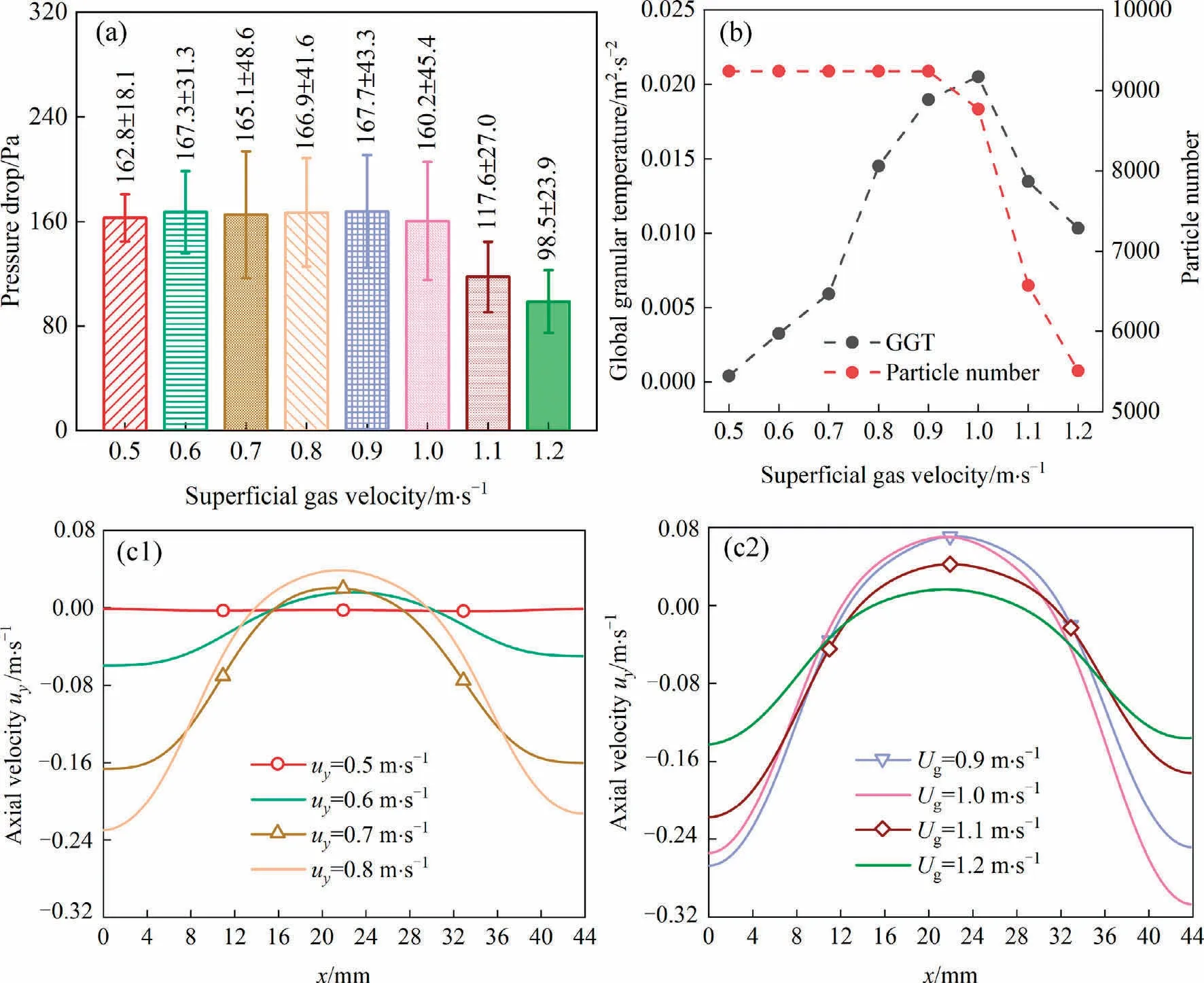
Fig.9.Comparison of (a) time-averaged pressure drop; (b) global granular temperature (GGT) and particle number; (c1, c2) time-averaged axial velocity in y direction.
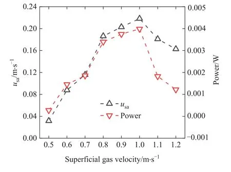
Fig.10.Comparison of time-averaged particle absolute velocity usa and timeaveraged interphase energy transfer rate.
The time-averaged pressure drops with different Ugare given in Fig.9(a).When the Ugis less than 0.9 m·s-1, the fluctuations of pressure drop are weak.As the Uggrows, the rapid decrease of pressure drop could be observed.This is related to the reduction of particle number.Particle numbers at 30.0 second are shown in Fig.9(b), as well as the GGT curve.Some particles escape from the simulation domain for the higher gas velocity.As the simulation scale is smaller than the experimental one,the escaped particles in the simulation could still stay in the fluidized bed.Thus,the case could not reflect the real gas-solid flow in which the Ugis greater than 0.9 m·s-1.But considering that few researchers reported the cases with reduced particle numbers,it is meaningful to further discuss the high Ugconditions.In the following discussion, the area where the Ugis less than 0.9 m·s-1is called the low-speed region, and vice versa is called the high-speed region.
As shown in Fig.9(c1) and (c2), uyincreases in the center and decreases near the wall with the growth of Ugin the low-speed region.At the beginning, the typical particle circulation is not significant at the height of 25 mm, with an almost constant uy.The raise of Ugresults in the strengthened circulation, whereas the velocity difference between the centre and wall at y = 25 mm is enlarged.From Figs.9(b) and 10, both usaand power increase rapidly, the same as GGT.This also shows that particle mixing is enhanced.All the above phenomena are attributed to the increased drag force.In a BFB, particle motion is mainly determined by drag force[78].The growth of Ugincreases the gas-solid relative velocity, resulting in the leap of drag force.The particle circulation is enhanced by the increased drag force.That is to say, the particles reach a higher position and fall back close the wall at a larger speed.
In the high-speed region, the trend is clearly different.When the speed changes from 0.9 to 1.0 m·s-1, the particle number decreases slightly from 9240 to 8770.The dominant position is still occupied by drag force, resulting in the mild growth of usa, power and GGT.When the speed changes from 1.0 to 1.1 m·s-1, the particle number is greatly reduced from 8770 to 6571.Furthermore,when the Ugis 1.2 m·s-1(4umf), 40.4% of particles would leave the domain.Larger uyat the center and smaller uynear the wall could be seen obviously from Fig.9(c2).At the same time, usa,power and GGT are greatly reduced.The situation is similar when the speed rises to 1.2 m·s-1.Affected by the growth of Ug, some high-speed particles leave the simulation domain, leading to the destruction of particle circulation.This is a situation that should be avoided during the simulation, because the simulation results are far from the real condition at this time.
4.Conclusions
Comparative analyses of drag models through plenty of MFIXDEM simulations are established based on the experimental and DNS results.Nine drag models are applied in the BFB for comparison.A series of indicators, including the pressure drop, voidage,angular velocity, granular temperature, and interphase energy transfer rate, are employed as the basis for evaluation.The impact of Ugon pressure drop, granular temperature, and axial velocity is also investigated.Conclusions are drawn as follows:
(1) Except for TGS and Wen-Yu models, the simulation results of drag models are consistent with the experimental and DNS data.The above two drag models are not suitable for the investigated BFB.The layer-by-layer particle movement is observed when using TGS drag model, leading to the abnormal transient results of interphase energy transfer rate, voidage profile, as well as the time-averaged results of axial velocity and granular temperature in y direction.The Wen-Yu drag model poorly predicts the time-averaged axial velocity and granular temperature at y = 35 mm.
(2) For all drag models,the time domain and frequency domain analysis of pressure drop are nearly the same.On the contrary, the angular velocity distributions obtained from all drag models are chaotic, without a unified law to explain the trend of the data.Based on the comparison of interphase energy transfer rate,predictions by BVK and Radl models are the closest to the DNS results.Gao and Sarkar models perform poorly, with the relative error of 110.6% and 103.2%,respectively.The performance of drag models derived from highly resolved TFM results is regrettable and unexpected.Consequently, it is recommended to use the drag model derived from DNS and fine grid CFD-DEM data first for CFD-DEM simulations in the BFB.Considering the influence of particle rotation could be a direction to improve the drag models.
(3) When the Ugis greater than 0.9 m·s-1(3umf), part of particles leaves the simulation domain.40.4% of particles have left while the Ugis 1.2 m·s-1(4umf).The decreased particle number leads to abnormal hydrodynamics in the investigated BFB.Therefore, the appropriate selection of the simulation domain size regarding Ugis essential for successful simulation.
Data Availability
Data will be made available on request.
Declaration of Competing Interest
The authors declare that they have no known competing financial interests or personal relationships that could have appeared to influence the work reported in this paper.
Acknowledgements
This work has been financially supported by the China-CEEC Joint Higher Education Project (Cultivation Project)(CEEC2021001).Srdjan Belošević, Aleksandar Milićević and Ivan Tomanović acknowledge the financial support by the Ministry of Science,Technological Development and Innovation of the Republic of Serbia (Contract Annex: 451-03-47/2023-01/200017).
Supplementary Material
Supplementary data to this article can be found online at https://doi.org/10.1016/j.cjche.2023.06.002.
Nomenclature
Subscripts
杂志排行

Chinese Journal of Chemical Engineering的其它文章
- Intrinsic kinetics of catalytic hydrogenation of 2-nitro-4-acetylamino anisole to 2-amino-4-acetylamino anisole over Raney nickel catalyst
- Experiments and model development of p-nitrochlorobenzene and naphthalene purification in a continuous tower melting crystallizer
- α-Synuclein: A fusion chaperone significantly boosting the enzymatic performance of PET hydrolase
- Influence of water vapor on the separation of volatile organic compound/nitrogen mixture by polydimethylsiloxane membrane
- Mass transfer mechanism and relationship of gas-liquid annular flow in a microfluidic cross-junction device
- Enhanced photocatalytic activity of methylene blue using heterojunction Ag@TiO2 nanocomposite: Mechanistic and optimization study