Study of limits to the rotation function in the SA-RC turbulence model

Wenho LI, Yngwei LIU,b,c,*

a School of Energy and Power Engineering, Beihang University, Beijing 100191, China

b National Key Laboratory of Science and Technology on Aero-Engine Aero-Thermodynamics, Beihang University, Beijing 100191, China

c State Key Laboratory of Aerodynamics, China Aerodynamics Research and Development Center, Mianyang 621000, China

KEYWORDS Non-equilibrium transport characteristics;Rotation and curvature correction;Rotation function;SA turbulence model;Separation flow;Tip leakage flow

Abstract The Rotation and Curvature (RC) correction is an important turbulence model modification approach,and the Spalart-Allmaras model with the RC correction(SA-RC)has been extensively studied and used. As a multiplier of the modelling equation’s production term, the rotation function fr1 should have a cautiously designed value range, but its limit varies in different models and flow solvers.Therefore,the need of restriction is discussed theoretically,and the common range of fr1 is explored in Burgers vortexes. Afterwards, the SA-RC model with different limits is tested numerically. Negative fr1 always appears in the SA-RC model, and the difference between simulation results brought by the limits is not negligible. A lower limit of 0 enhances turbulence production,and therefore the vortex structures are dissipated faster and shrink in size,while an upper limit plays an opposite role.Considering that the lower limit of 0 usually promotes the simulation accuracy and fixes the numerical defect, whereas the upper limit worsens the predictive performance in most cases, it is recommended to limit fr1 non-negative while utilizing the SA-RC model. In addition, the RC-corrected model has a better prediction of the attached flow near curved walls, while the SA-Helicity model largely improves the simulation accuracy of three-dimensional large-scale vortices. The model combining both corrections has the potential to become more adaptive and more accurate.

1. Introduction

The rapid growth of computing power enables high-accuracy simulation methods such as Direct Numerical Simulation(DNS), Large-Eddy Simulation (LES), and Detached Eddy Simulation (DES) to be utilized in scientific research. However, the fundamental Reynolds-Averaged Navier-Stokes(RANS) method will still be widely used in future decades.1The accuracy of RANS simulation relies on the performance of turbulence models which mainly include Reynolds Stress Models (RSMs) and Eddy-Viscosity Models (EVMs). Considering the low robustness and high computation cost of RSMs, conventional EVMs still have high research value.

Among them,the Spalart-Allmaras(SA)model2is a classical one-equation turbulence model. Its modelling equation reflects a more sophisticated turbulence transport mechanism than those of primitive mixing length models. Compared with two-equation EVMs, the SA model is more robust and costs fewer computing resources. Therefore, the SA model is still deeply studied and widely used at present.3-7Based on different flow structures and physical mechanisms, researchers have proposed various modifications of the SA model to promote its predictive performance. One type of modification introduces nonlinear and anisotropy effects. For example, the SAQCR2000 model1adds a quadratic term to the original Boussinesq assumption and shows improvements in predicting the secondary flow within a square duct. Based on SAQCR2000, the SA-QCR2013 model5has an estimation of the-2ρk/3 term in Reynolds normal stresses and performs well in simulating secondary flows in sharp corners.The other type of modification which is studied emphatically focuses on the non-equilibrium transport characteristics. For instance, Liu et al.3put forward the SA-Helicity model which firstly considers the effect of turbulence energy backscatter using helicity,and it greatly promotes the performance in predicting vortical flows such as the corner separation and the tip leakage flow.8-11The modification concept also significantly improves the stall margin simulation accuracy of fans.6,12-13Based on pressure gradient, Ma et al.14proposed an SA model correction which shows superiority in simulating shock-wave/boundary layer interaction flows.

In the equation of the SA model, it is a consensus that the production term should never go negative.4,26-28As for the aforementioned SA-RC model, its rotation function fr1is directly multiplied by the production term, and thus the value range of fr1must be chosen cautiously. At first, the RC correction has no limit to fr1in reference and when it was originally designed for the SA model.19,29Spalart and Shur19discovered that fr1is negative somewhere in the flow field which results into negative production of the turbulent viscosity. However, they left it alone since they determined that the effects of negative production on the turbulent eddy viscosity and the mean flow field are weak. Afterwards, in the SST-RC model, a lower limit of 0 is given to fr1for numerical stability reasons. An upper limit of 1.25 is also introduced to prevent excessive turbulence production, since the strain rate S-based production term of SST is generally larger than the vorticity Ω-based one of SA.24Then, in ANSYS Fluent, the [0, 1.25] limit to fr1is adopted in the correction options for both SA and two-equation EVMs.A strict limit to fr1in the SA-RC model enhances numerical stability, but the upper limit of 1.25 may not be suitable since it is designed for the strain rate S-based production terms of two-equation models. The necessity of a lower limit should also be discussed.

Consequently, based on the SA-RC model,the value range and suitable limit of the rotation function fr1are deeply studied in this work. Firstly, starting from turbulence modelling theories and numerical simulation experience,the limit to fr1is analyzed theoretically as a multiplier by the SA model’s production term. Secondly, to find out the common value range, fr1is calculated in a series of analytical flows which include the Burgers vortex30and its superposition with shear flows. Thirdly, after adopting different limits to fr1, the resulting SA-RC models are validated in cases including classical two-dimensional flows such as the wall-mounted hump, the U-duct, and the axisymmetric transonic bump. Realistic three-dimensional flows such as the corner separation flow and the tip-leakage flow within an axial compressor are also simulated. Taking experimental data and high-accuracy simulation results as references, different SA-RC models are compared in detail to find out an appropriate limit range of the rotation function fr1.Modification in the SA-Helicity model is also validated which helps to propose a more adaptive model.

2. Theoretical analysis of rotation function

2.1. Rotation and curvature corrections

As the main target studied in this work,the SA-RC model is a modification to the SA model2whose modelling equation about the turbulent viscosity ν～is

and the constant cr2is changed to 2.0.In Eq.(15),ω stands for the specific dissipation rate provided by the turbulence modelling equation.

In commercial software ANSYS Fluent25, the RC option can be enabled in the SA model as well as in two-equation EVMs. However, in the option for SA, the rotation function fr1is also limited in the range of[0,1.25]like in Eq.(13),which is different from SA-RC in references. The limit enhances numerical stability, but its necessity and influence on simulation results should be evaluated in detail.

2.2. Limit to SA model’s production term

and the constant cv2equals to 5.0.Although the SA-fv3 model has defects in simulating transition flows at low Reynolds numbers26, it still indicates that the production term should be strictly non-negative.

and constants c2and c3are 0.7 and 0.9, respectively. As S-/Ω decreases, S～/Ω decreases progressively to 0.1 in this new definition, and the trend is shown in Fig. 14. Unlike the original S～/Ω which goes negative when S-/Ω ＜-1, the new model ensures that S～/Ω is always positive. It should be noted that the authors believe that only S～/Ω ＞0.3 complies with physics,which is in consistent with the theory proposed by Spalart26.

For the same problem,Rumsey28noted that the SA model’s production term must be greater than zero to avoid numerical problems.Three optional solutions are proposed:(A)limit the production term to be greater than zero directly which is the easiest way; (B) limit S～to be no less than 0.3Ω; (C) utilize the progressive form of S～put forward in Ref.4as above.

Since the SA model was originally designed, it has had the ability to deal with laminar flow and transition.These extreme situations even occur in a flow field with a fully turbulent inlet boundary condition at high Reynolds numbers (such as in the boundary layer). A particular treatment called ‘‘blanking” is often used to deal with laminar regions in turbulent flow simulations.26One kind of blanking solves the turbulence modelling equation as usual, but the turbulent eddy viscosity μTis not used in momentum and energy equations. This method may face risks since the turbulence modelling equation is designed in a closed system together with the RANS equations.The other way of blanking forces the production term of the turbulence modelling equation to be zero.Anyway, a negative production term should never exist even in laminar regions of the flow field.

Fig. 1 Variation of S～/Ω along with S-/Ω.4.

The RC correction is a modification method from the aspect of non-equilibrium transport characteristics. Apart from classical turbulent flow structures such as wall boundary layer, mixing layer, and wake, the correction should also be suitable for more complex situations.For example,the correction in the SA-R model22which has a similar purpose to the RC correction suppresses turbulence production in pure rotation regions.Accordingly,S～in the production term is modified into

where Crot=2.0 is a constant. Regardless of the last term in Eq. (21) which is very small away from the solid wall boundary, it is easy to find that S～will go negative when Ω ＞2S.For this reason, numerical problems caused by the modified model are encountered in the core region of a vortex.22Consequently, in the widely used flow solver CFL3D33, the production term (S～) is still limited to be non-negative in the SA-R model.

Overall, under no circumstances should the production term (S～) go negative. A lower limit of 0 is necessary for the rotation function fr1in the RC correction theoretically. In addition, it is better to take into consideration the physical restriction that S～should be larger than 0.3Ω.

2.3. Rotation function fr1 in Burgers vortex

Describing an isolated vortex, the classical Burgers vortex30is an exact solution to the Navier-Stokes equations. It can be used to model tubular structures in turbulent flows, and be taken as a reference for experimental observations.34It is also an important mathematical model in the research of vortex structures and stability.35In addition, the Burgers vortex can be superposed with other flows to extend its application.Among the realistic flow cases studied in this work, the Tip Leakage Vortex (TLV) has features in common with those of the Burgers vortex.36Two- and three-dimensional separated flows which contain a separation vortex can also get inspiration.

A Burgers vortex describes an incompressible timeindependent axisymmetric flow field whose velocity components in a cylindrical coordinate （r， θ， z） are

where Γ is the circulation, A is the axisymmetric strain rate,and ν stands for the molecular kinematic viscosity. Two key parameters are selected to define a Burgers vortex: one is the Reynolds number Re=Γ/2πν and the other is A/ν where ν is set to 1.5 × 10-5m2/s in the following cases. A twodimensional slice in the flow field is analyzed,with coordinates ranging from-0.5 m to 0.5 m.Moreover,the rotation function fr1is calculated from the flow field variables using the formula of SA-RC.Fig.2 shows the variation trends of maximum and minimum fr1in the domain according to different Re and A/ν.It is found that the minimum value maintains at -2.37 when Re ＞100 and A/ν ＞10, while the maximum value maintains at 3.46 when Re ＞10000 and A/ν ＞100.

Fig. 2 Variation of fr1 with Re and A/ν in Burgers vortexes.

As examples, the vorticity and fr1in three Burgers vortexes under different flow conditions are shown in Fig.3 and Fig.4,respectively. When Re and A/ν get larger,the vortex structure remains the same, but the vortex core gets concentrated and can be fully captured within the domain. It can also be found that vorticity in the core is proportional to the product of Re and A/ν. As shown in Fig. 4, fr1is negative in the inner part of the vortex while positive in the outer part. This explains the variation trends of maximum and minimum values in Fig. 2.Firstly, when Re and A/ν are very small, the minimum fr1decreases as the vortex gets concentrated. Then, the minimum value gets fixed(Re ＞100,A/ν ＞10),and the maximum fr1is still growing.Finally,the vortex is thoroughly captured in the domain, and the value range of fr1never changes(Re ＞104, A/ν ＞100). In conclusion, the rotation function fr1ranges from -2.37 to 3.46 in the Burgers vortex, and the right-most condition (Re=105, A/ν=200) in Fig. 3 and Fig. 4 is representative.

where u, v and w are the velocity components of the shearing motion, r～0 =1.5852 is the non-dimensional vortex size38, and C is a user-specified constant which is set to 1 and -1 in this work.After applying the shear component,the streamline curvature has made a big change, and this analytical model can represent more flow situations. When C=1, the vorticity becomes larger compared with that of a pure vortex, and the streamlines are flatter as shown in Fig. 5. fr1ranges from -1.68 to 3.02, with the minimum increasing and the maximum decreasing compared with those of the baseline case. As in Fig. 6, when C=-1, the vorticity of the Burgers vortex and the uniform shear flow offset each other. Negative vorticity occurs in the outer region of the vortex,and the flow structure totally changes under the shearing effect.In this case,the range of fr1is from -2.89 to 8.03 which gets much wider. Large positive values appear on both sides of the core region,and negative values are distributed around. In all the above cases,negative fr1always appears and is widely distributed.

3. Numerical methods

3.1. Turbulence models

Considering the wide range of fr1,a limit such as[0,1.25]in the RC option of Fluent may influence the predictive performance of the SA-RC model.From preceding studies,it is common for fr1to be negative while the production term should be limited non-negative according to physical requirements. Thus, a lower limit of 0 seems reasonable,but the influence during simulation still needs to be evaluated. Besides, the upper limit of 1.25 is designed for the strain rate S-based production terms of two-equation EVMs,and may not be suitable for the vorticity Ω-based production term of the SA model.Even the necessity of an upper limit in the SA-RC model needs to be discussed.

Therefore,a series of SA-RC models with different limits to the rotation function fr1is tested in comparison with the original SA model, experimental data, and high-accuracy simulation results. As listed in Table 1, the models studied include the original SA-RC model, the SA-RC-min0 model with a lower limit of 0, the SA-RC-max1.25 model with an upper limit of 1.25, and the SA-RC-min0-max1.25 model with a [0,1.25] limit.

Fig. 3 Distribution of vorticity in Burgers vortexes.

Fig. 4 Distribution of fr1 in Burgers vortexes.

Fig. 5 Distributions of vorticity and fr1 when Re=105, A/ν=200, and C=1.

Fig. 6 Distributions of vorticity and fr1 when Re=105, A/ν=200, and C=-1.

Inaddition,the SA-Helicity model3is also validated and used as a reference in three-dimensional flow cases,since it reflects different modelling ideas from the RC correction but is passive in two-dimensional conditions.It is expected to provide different simulation results and inspiration for turbulence modelling.In the SA-Helicity model,the formulation of S～is modified into.

Table 1 Limits to fr1 in tested SA-RC models.

The model constants Ch1and Ch2are 0.71 and 0.6, respectively. It is obvious that H equals to zero in two-dimensional conditions, and the model degenerates to the original SA model.

3.2. Testing platform

In this work, RANS simulations utilizing various turbulence models are conducted with the open-source code CFL3D.33The flow solver is based on a structured-grid and finitevolume method.After modifications,the code is more applicable to internal flow simulations and has more optional turbulence models. In the following RANS cases, a third-order upwind-biased spatial discretization scheme and a first-order implicit time advancement scheme are used.

4. Simulation results and discussion

4.1. NASA wall-mounted hump

Fig. 7 Model of NASA wall-mounted hump39.

Separated flow over a NASA wall-mounted hump(Fig. 739)is a typical two-dimensional flow whose main features are the curved lower wall and the resulting adverse pressure gradient.The reference velocity of this low-speed separated flow Urefis about 34.6 m/s(Mach number Ma=0.1).Based on this flow,detailed experimental results were provided by Greenblatt et al.39-40and Naughton et al.41. In terms of numerical simulations, Rumsey et al.42considered the hump separation as a challenging case for RANS methods after reviewing abundant RANS results.By comparison,high-accuracy simulations perform better, such as the LES data presented below and provided by Uzun and Malik43. In this work, the grid used during numerical simulations has been confirmed fine enough after independence verification among different grids provided on the NASA Turbulence Modeling Resource website28.It has 817 points streamwise and 217 points normal,which is 177289 points in total.

The positions of separation and reattachment points which reflect the separation size are the most important parameters in evaluating simulation accuracy. Extracted from the results of different models,separation/reattachment positions are identified according to the wall friction coefficient and compared in Table 2.In addition,the length of the separation region is also calculated and used for evaluating the relative error. It can be found that the LES slightly underestimates the separation size,while the RANS models overestimate it. Compared with the experiment, separation happens a little earlier, and reattachment is largely delayed in all RANS results. However, four SA-RC-based models give different results, and their difference is not negligible compared with that between the original SA model and the SA-RC model.In other words,with limit to fr1, the SA-RC model performs like a new version of the SA model, and thus the limit range should be chosen carefully.As shown in Fig.8,fr1ranges from-3.25 to 9.19 in the originalSA-RC model; therefore, it is not strange that these limits make such a difference.

Table 2 Comparison of simulation results (NASA wall-mounted hump).

Fig. 8 Distribution of fr1 in NASA wall-mounted hump.

Among the RANS models, SA-RC shows improvement over the original SA, and SA-RC-min0 performs the best. In contrast, SA-RC-min0-max1.25 decreases the accuracy of SA-RC, and SA-RC-max1.25 performs the worst. Overall,the RC correction is effective in this case by reducing the separation size.In addition,the lower limit of 0 improves the performance,while the upper limit of 1.25 worsens it.In different SA models, the length of the separation region is mainly affected by the magnitude of the turbulent eddy viscosity μT.If the turbulence production is enhanced, the general level of μTwill increase, and thereby the separation region will shrink in size owing to stronger dissipation. The opposite is also true when the turbulence production is suppressed. Therefore, on the basis of the SA-RC model, the lower limit to the production term reduces the separation size and promotes model accuracy, while the upper limit plays an opposite role.

By comparing the separation and reattachment positions,a strange phenomenon is that the separation region of the SARC model shrinks in size, but the separation point moves upstream (deviates more from the experiment) compared with the original SA model. This is attributed to the turbulent viscosity distribution and the related momentum transport inside the boundary layer. Fig. 9 shows the distributions of fr1, the turbulent viscosity ν～, and the streamwise velocity U/Urefnear the lower wall at x/c=0.65. This axial position is located on the convex hump, a little ahead of the separation point. Since the RC correction is designed to enhance turbulence production on a concave surface and to suppress it on a convex one17,19,fr1is less than 1 near the wall (y+＜50). Thus ν～of both SA-RC and SA-RC-min0 in this region is smaller than that of the original SA model. Above this region, fr1is larger than 1, and ν～of the SA-RC and SA-RC-min0 models grows faster than that of the SA model. However, fr1of the SA-RC model goes negative from y+≈600, while the SA-RC-min0 model with a lower limit of 0 avoids negative production here which is still in the boundary layer. As a result, the SA-RCmin0 model finally reaches a larger ν～than that of SA-RC,thereby the momentum transport is enhanced. The velocity profile becomes fuller in the boundary layer, and the ability to resist separation gets stronger.In conclusion,the lower limit in the SA-RC-min0 model fixes the negative production of SARC over a convex surface, and therefore avoids the issue that separation happens in advance.

4.2. U-duct

Flow in a U-duct is characterized by the separation at the sharp U-turn, and is widely used for RC correction studies.The geometry and corresponding coordinates of the U-duct model are shown in Fig. 10, where h represents for the duct height, φ represents for the central angle and s is the streamwise distance.In this paper,the Reynolds number of the studied flow condition is about 106, based on the channel width and bulk velocity at the inlet. Additionally, experimental results provided by Monson et al.44are displayed for comparison.A series of grids is generated to examine the grid independence, which has 5 × 104, 1.9 × 105, and 7.6 × 105points in total. By comparing the flow field details, the 1.9 × 105grid(633 points streamwise and 301 points normal) is verified to be fine enough and therefore used for subsequent computations.

As shown in Fig. 11, fr1given by the SA-RC model ranges from -2.71 to 7.72 in this case. At the U-turn, positive fr1values mainly occur near the outer wall, and negative values are distributed near the inner wall. This agrees with the theory of RC correction that turbulence production should be suppressed near a convex surface and enhanced near a concave one.17,19As for the predictive performances of different models, separation and reattachment positions are extracted from the inner wall friction coefficient and compared with the experiment44in Table 3.It can be found that the original SA model performs the best especially in terms of the separation size. In contrast, the SA-RC-based models have better predictions of the separation point, but their reattachment positions are much delayed. The separation size is largely overestimated by these SA-RC models. Compared with SA-RC and SA-RCmax1.25, SA-RC-min0 and SA-RC-min0-max1.25 predict slightly delayed separation but more accurate reattachment points. Again, the lower limit of 0 shortens the separation region and obviously improves the model performance. On the contrary, the upper limit of 1.25 enlarges the separation region by bringing forward the separation point as well as postponing the reattachment point.

Fig. 9 fr1, ν～and U/Uref near lower wall at x/c=0.65.

Fig. 10 U-duct model and corresponding coordinates.

Fig. 11 Distribution of fr1 in U-duct.

Near the reattachment point where the tested models show large differences, distributions of the streamwise velocity U/Urefdownstream from the U-turn at x/h=2 and x/h=4 are presented in Fig.12.Overall,the RANS models fail to predict a recovery of the velocity profile, whereas the original SA model is relatively accurate among them.At x/h=2,the flow has already reattached in the experiment as well as in the result of the SA model. On the contrary, there still exists backflow near the inner wall in the results of the SA-RC models owing to the delayed reattachment. The advantage of the SA-RC models is that their velocity profiles fit relatively well with the experiment near the outer wall. Since the turbulence production is enhanced near the concave surface, the velocity in the boundary layer becomes higher which is close to the experimental data. Among the SA-RC models, the SA-RC-min0 model has the smallest backflow region and the lowest main flow velocity which performs the best. It can be found that the lower limit of 0 always promotes the simulation accuracy while the upper limit of 1.25 worsens it by delaying the recovery of backflow. As shown in Fig. 12(b), the performance of each model basically remains the same at x/h=4 except that the flow has reattached in all simulation results. The SA-RC models still have better prediction of the boundary layer near the outer wall (concave wall) than that of the SA model, but the prediction on the inner wall side is inaccurate.

The SA-RC models show advantages against the SA model in simulating the position of the separation point and the velocity distribution in the concave wall boundary layer,which indicates a success of RC correction in predicting attached flow near curved walls. However, since the rotation function fr1is derived based on the precondition of weak rotation or curvature19, it has difficulty in accurately describing the turbulence characteristics of the strong rotating flow in the separation region, and this leads to an overprediction of the separation region length.Near the inner wall(convex wall)of the U-turn, negative turbulence production appears again which can be found in Fig. 11. Therefore, the lower limit of 0 takes effect to enhance turbulence production. Moreover,the higher level of the turbulent viscosity in the result of SA-RC-min0 reduces the size of the separation region, while the upper limit plays an opposite effect. Consequently, the SA-RC-min0 model gets a much better result than that of the SA-RC model.

4.3. Axisymmetric transonic bump

The axisymmetric transonic bump flow is a transonic case,which considers an axisymmetric separated flow triggered by shock-wave and adverse pressure gradient. The freestream Mach number of this flow is 0.875, and the Reynolds number based on the bump length is 2763000. Based on this flow,abundant experimental data was provided by Bachalo and Johnson45-46, while Johnson et al.47-50conducted various RANS simulations. In terms of high-accuracy simulations, a DNS-IDDES(Improved Delayed Detached-Eddy Simulation)hybrid method was utilized by Spalart et al.51, and a wallresolved LES was done by Uzun and Malik52which is taken as the reference here.They both get more accurate results than those of RANS simulations.

Table 3 Comparison of simulation results (U-duct).

Fig. 12 Distributions of U/Uref in U-duct.

Corresponding experiments are carried out in 2 ft × 2 ft(1 ft = 0.3048 m) and 6 ft × 6 ft wind tunnels. However,due to the relatively larger influence of tunnel walls in the 2 ft × 2 ft tunnel, results from the bigger tunnel are considered more valid.52To be in line with the LES settings in Ref.52,the outer boundary is located at r/c=10.0 (Fig. 13) and set as Riemann far field in this work.Besides,the flow is simulated using a two-layer mesh with rotational periodic interfaces.The computational grid contains 721 points streamwise and 361 points normal, which is totally 260281 points. Meanwhile,the grid independence has also been verified.

Compared with the experiment48-49and LES52result in Table 4, the original SA model performs the best in terms of reattachment position and separation size. The SA-RC-min0 model has the closest separation position to that of the LES,which indicates the advantage of RC correction on simulating attached flow over curved wall. However, the SA-RC models all predict an oversized separation region by largely postponing the reattachment,owing to their lower accuracy in the separation region. In the result of the SA-RC model, fr1ranges from -3.26 to 9.18 which is still very wide, and therefore the simulation result shows sensitivity to different limits. The lower limit of 0 plays a positive role in SA-RC-min0 and SA-RC-min0-max1.25 by shortening the separation size,which is in consistent with its effect in the other two-dimensional cases. On the contrary, SA-RC-max1.25 and SA-RC-min0-max1.25 are less accurate because of the upper limit.

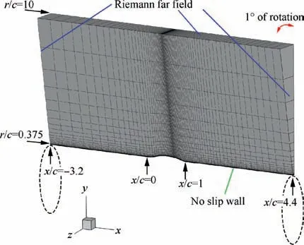
Fig. 13 Grid and settings of axisymmetric transonic bump(every eighth grid line is shown).

Table 4 Comparison of simulation results (axisymmetric transonic bump).

Negative effect caused by the lack of a lower limit to turbulence production appears again on the bump surface. Compared with the separation point in the LES (x/c=0.679),the SA-RC model predicts an earlier separation(x/c=0.671),while the SA-RC-min0 model is relatively more accurate(x/c=0.675).Fig.14 shows the distributions of fr1,ν～,and U/Urefabove the bump at x/c=0.67 (just before separation). It can be found that the SA-RC model predicts a negative fr1region in the boundary layer (300 ＜y+＜700) over the convex surface. After applying a lower limit of 0, fr1given by SA-RC-min0 increases obviously. Therefore, the turbulent viscosity ν～of SA-RC-min0 is always greater than that of SA-RC.The velocity profile gets fuller under stronger momentum transport, and the separation point moves downstream.

Fig. 14 fr1, ν～and U/Uref near solid boundary at x/c=0.67.

Fig. 15 Shock-wave and static pressure coefficient on solid wall.

Apart from the separation region,there also exists a shockwave over the bump, which should also be accurately simulated. In the static pressure distribution shown in Fig. 15 (a),a shock-wave can be observed.In addition,each line of the surface static pressure coefficient Cpin Fig.15(b)has an inflection point between x/c=0.6 and x/c=0.7,which can be regarded as the axial position of the shock-wave.It is found that the LES fits well with the experiment in terms of surface static pressure coefficient especially near the position of the shock-wave, and there is a distance between the shock-wave (x/c ≈0.6) and the separation point (x/c=0.679). In contrast, the shockwave is located downstream in all RANS results, and its position is only a little ahead of the corresponding separation point regardless of whether RC correction is used or not, which means that the model predicting a later separation always provides a less accurate shock-wave position. For example, the shock-wave in the original SA model deviates the most from the experiment, while SA-RC-max1.25 and SA-RC-min0-max1.25 perform relatively well in static pressure coefficient prediction. Considering that the RC correction mainly affects the turbulence transport characteristics within the curved wall boundary layer and the separation vortex, it is believed that the absence of a certain mechanism (the interaction between the shock-wave,the turbulent boundary layer,and flow separation)in the SA model results in the inability of predicting both the shock-wave and flow separation accurately.

4.4. Linear cascade

Except for two-dimensional flows, three-dimensional corner separation flow in a linear highly-loaded Prescribed Velocity Distribution (PVD) cascade53is studied as a representative of complicated three-dimensional separations. The massive three-dimensional separation is still a challenge to RANS models.54In this low-speed compressor cascade, the reference velocity at the inlet is 23.82 m/s (Ma ≈0.07). Other geometric and aerodynamic parameters are listed in Table 553.

As shown in Fig. 16, an O4H grid of the cascade is generated with about 1.5 million grid points in total and 81 layers spanwise. The height of the first grid line to the solid wall is y+≈0.7, and this computation grid is confirmed fine enough after grid independence verification.10To reduce the simulation cost,the domain covers half of the span after introducing a symmetrical plane. The flow condition under zero incidenceis studied according to available experimental data53. Besides,the velocity profile from the experiment is specified at the inlet,and the static pressure at the outlet is set to 101325 Pa.

Table 5 Parameters of linear PVD cascade.53

Fig. 16 Mesh topology and boundary conditions of PVD cascade.

To evaluate the flow loss of the corner separation flow,the total pressure loss coefficient Cptis calculated from

where P01stands for the reference total pressure at the inlet,P1is the reference static pressure, and P0is the local total pressure. On the measurement slice which is located at 50 % of the axial chord length behind the trailing edge, the distributions of Cptand fr1given by the SA-RC model are shown in Fig.17,where the high Cptarea indicates the corner separation region. fr1ranges from -2.41 to 7.44 on this slice, and from -3.21 to 8.80 in the whole domain. The wide range from a negative value to a large positive one is quite common for the rotation function.

Fig.18 shows the Cptdistributions of various models on the measurement slice. Compared with the experiment, the original SA model largely over-predicts the corner separation region and the peak Cpt. There is only a tiny area that Cptis over 0.6 in the experimental data, while it is generally larger than 0.75 in the core zone as in the result of the SA model.The SA-RC models get even higher Cptthan that of the original SA model at the center of the separation region which is over 0.8, and the difference in the Cptdistribution brought by the limits to fr1is not very large. The upper limit of 1.25 slightly enlarges the high-loss region.Near the mid-span(highlighted with red boxes), the flow is approximately twodimensional, and therefore the influence regularity of limits to fr1is similar to previous conclusions in two-dimensional flows. After applying the lower limit 0 (SA-RC-min0 and SA-RC-min0-max1.25), the width of wake and the flow loss in it both decrease, since the turbulence production is enhanced and the two-dimensional separation vortex shrinks.On the contrary,the upper limit of 1.25 results in a wider wake region, and the flow loss increases accordingly.

Fig. 17 Corner separation region and fr1 on measurement slice.

As a model modified for three-dimensional large-scale vortices,the SA-Helicity model slightly underestimates Cpt,but its shape of the separation region is the closest to the experiment.Since the RC correction especially SA-RC-min0 shows improvement in predicting two-dimensional attached flow, a combination of SA-Helicity and SA-RC-min0 has the potential to become a more adaptive model. Considering that the helicity correction is inactive under two-dimensional conditions, the combination is feasible and clear in mechanism.From the distribution of Cpt, the SA-Helicity-RC-min0 model has a slightly lower value than that of SA-Helicity.

Fig.19(a)shows the mass-averaged Cptalong the span.The result of the SA-Helicity model fits the best with the experiment except that Cptat 65 % to 85 % of the span is underestimated. In comparison, the SA-Helicity-RC-min0 model provides a little higher value near the mid-span and a little lower value near the blade root. Simulation results of other models are all much higher than that of the experiment.Compared with the original SA model, the SA-RC models get higher Cptnear the mid-span but show slightly lower values around 70 % of the span, and their Cptlines are very similar to each other. Considering that the SA-RC models have obviously higher peak values of Cpt(as shown in Fig.18),their separation regions are necessarily more concentrated in size, and the situation is more severe in SA-RC-max1.25 and SA-RCmin0-max1.25 due to their even larger high-loss regions.Fig.19(b)shows the spanwise distribution of the outflow angle on the measurement slice. The SA-Helicity and SA-Helicity-RC-min0 models have very accurate predictions, and SAHelicity-RC-min0 provides a slightly larger outflow angle near the mid-span which fits better with that of the experiment.Other models get much higher values since the oversized separation region pushes the main flow away from the blade suction surface. Among them, the SA-RC and SA-RC-min0 models perform slightly worse than the original SA model at both the mid-span and the corner separation region, but they still show superiority over SA-RC-max1.25 and SA-RCmin0-max1.25 from 80 % to 95 % of the span.

Overall, the original SA model largely overestimates the three-dimensional corner separation region, while the SAHelicity model can accurately simulate the airflow deflection and associated flow loss. The combined model SA-Helicity-RC-min0 retains the predictive performance of SA-Helicity,and also provides accurate results. It is believed that the RC correction is not as effective as the modification of SAHelicity in corner separation flow.Compared with the original SA model, SA-RC and SA-RC-min0 are less accurate by simulating higher peak values of Cptand larger outflow angles,but they are still better than SA-RC-max1.25 and SA-RC-min0-max1.25.The lower limit of 0 has little influence on the result,but it improves the simulation accuracy near the mid-span. In fact,for many versions of the SA model,the flow loss of corner separation in the PVD cascade under zero incidence is either quite small as that of the SA-Helicity model or very large as that of the original SA model. A medium value in between is hardly found. It is the same case while conducting coefficient studies on the SA model. The reason is that, along with an increasing incidence, corner separation in the highly-loaded PVD cascade turns into corner stall, and a critical incidence exists around 2°.The corner separation flow becomes destabilized, and the flow loss suddenly increases consequently.Therefore, Cptwill become very large if the turbulence model judges the flow under zero incidence as corner stall, which is the situation of the original SA model and the SA-RC models.

Fig. 18 Predictions of Cpt by different models.

4.5. Axial compressor rotor

The low-speed large-scale axial compressor55at Beihang University simulates the back stages of a high-pressure compressor based on the similarity theory. The blade height is enlarged to 200 mm, and the Mach number at the rotor inlet is around 0.08. Within this compressor, the rotor tip leakage flow has been studied experimentally using stereoscopic particle image velocimetry.55Besides, it has also been studied numerically for turbulence modelling research and highaccuracy simulations.56-57The geometric and aerodynamic parameters of this compressor are shown in Table 6.55

Considering that the large axial gaps between blade rows weaken the unsteady blade row interactions and multirow full-annulus unsteady simulation with a highly-resolved grid is still too expensive, only an isolated rotor is simulated to evaluate the model performance for the tip leakage flow. This also avoids errors from the adjacent blade rows by steady multirow simulation with the mixing-plane method. For clearer comparison, a larger tip gap (3.5 mm) is chosen to obtain a conspicuous TLV.As shown in Fig.20,an O4H grid is generated with about 2.6 million grid points in total, and the distance from the first grid line to the solid wall is y+≈0.9.The grid independence has been verified by assessing the flow structures in the tip region among a series of grids with different densities and distributions.36In terms of boundary conditions, the distributions of total temperature, total pressure,and flow angles measured in the experiment are specified at the inlet, while the radial pressure equilibrium condition at the outlet is adjusted for different operating conditions.

Fig. 19 Distributions of Cpt and outflow angle along span.

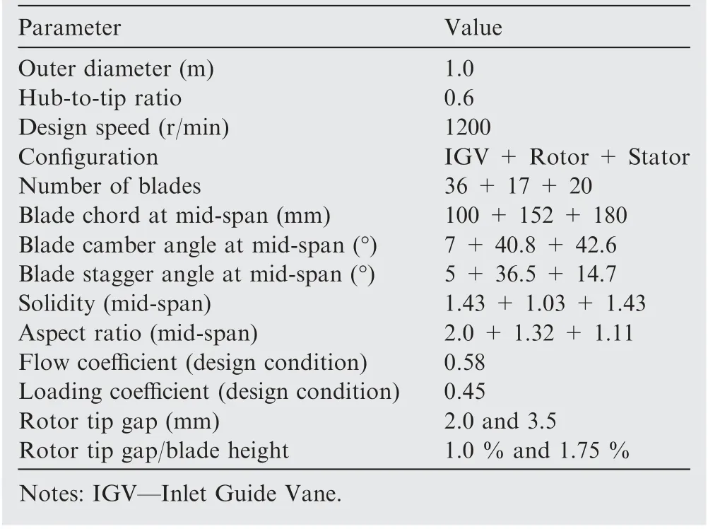
Table 6 Parameters of axial compressor.55

Fig. 20 Mesh topology of isolated rotor.

Fig. 21 shows the operating characteristics given by Delayed Detached-Eddy Simulation (DDES)58and various SA models, in which the static pressure rise coefficient Cpand the mass flow coefficient φ are defined as

Fig. 21 Operating characteristics of pressure rise coefficient.

where Poutand Pinare the averaged static pressures at the outlet and the inlet,respectively,ρ stands for the reference density,Vmidis the rotor mid-span circumferential speed,and Vaxial，inis the mass averaged axial velocity at the inlet. Although the Cpdata of the isolated rotor is not available in the experiment,the high-accuracy result of DDES is compared to evaluate the predictive performance of RANS models. In terms of the stall margin, φ at the stall point is 0.485 in the experiment. Owing to high computation cost, the DDES result simulates a nearstall condition at φ=0.509 instead of going further towards the stall point. As for RANS simulations, the back pressure at the near-stall point approaches less than 1 Pa away from numerical divergence. Compared with the experiment and the DDES result, the original SA model underestimates the stall margin as well as Cp, while the SA-RC models perform even worse. In contrast, the prediction accuracy of the SAHelicity model is significantly better than that of the SA model.The operating characteristic of the SA-Helicity-RC-min0 model lies between the results of SA-Helicity and SA-RCmin0, which is close to that of the original SA model. In the result of the SA-RC model, the rotation function fr1ranges from -2.92 to 7.87 under the design condition in the whole domain, which is still in line with the typical range. With the upper limit of 1.25, the SA-RC-max1.25 and SA-RC-min0-max1.25 models can reach lower φ at near-stall condition than those of SA-RC and SA-RC-min0.Oppositely,the lower limit of 0 slightly worsens the stall margin prediction which can be found by comparing SA-RC-min0 with SA-RC (or SA-RCmin0-max1.25 with SA-RC-max1.25), but it results in higher Cpespecially under low-mass flow conditions.Overall,judging from the operating characteristics, the upper limit of 1.25 is beneficial for stall margin prediction, while the lower limit of 0 provides more accurate Cp.

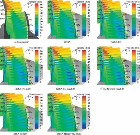
Fig. 22 Distributions of streamwise velocity under design condition.

As for the design condition at φ=0.58,the SA-RC models severely underestimate Cpcompared with DDES and other models. Among them, SA-RC-min0-max1.25 has relatively the best prediction of Cpwhich is a little higher than that of SA-RC-min0, while SA-RC and SA-RC-max1.25 perform the worst. Therefore, at the design condition, the lower limit of 0 improves the prediction accuracy of Cp, and the upper limit of 1.25 also has a little positive effect. For detailed comparison, Fig. 22 and Fig. 23 show the streamwise velocity and streamwise vorticity on measurement slices under the design condition, respectively. Compared with the experiment, the original SA model predicts a stronger velocity loss especially at the downstream part of the TLV. In terms of the vorticity distribution, the influence area of the TLV lasts until 95 %of the chord length on the pressure side since the vortex is dissipated very slowly. With a strong TLV, recovery of the pressurizing ability in the blade channel becomes harder, and therefore Cpis obviously underestimated by the SA model.In contrast, all SA-RC models receive an even stronger TLV in terms of both the velocity loss and the vorticity magnitude,because the RC correction makes the quasi rigidly-rotating TLV more stable and harder to be dissipated. This explains the much lower Cpgiven by the SA-RC models than that of the SA model. Differently, the SA-Helicity model enhances turbulence production in the TLV region, and therefore the vortex is dissipated faster. Its velocity loss is significantly weaker than that of the SA model, and is closer to the experiment. From the perspective of vorticity distribution, the predicted TLV strength is weaker than that of the SA model,and the positive vorticity part next to the TLV is more similar to the experimental result. Similarly, the combined model SAHelicity-RC-min0 also simulates a relatively weak TLV. The level of velocity loss is close to the result of the SA-Helicity model, but the negative vorticity region is slightly larger.

In the vorticity distribution of the experimental result, the negative vorticity at the core during the initial stage (30 %to 70 % of the chord length on the suction side) is very obvious, and then the TLV dissipates quickly. Actually, the TLV becomes unstable and breaks down when it develops downstream, and this unsteady process cannot be captured in RANS simulations. Therefore, it is difficult for a turbulence model to accurately simulate every stage of the TLV development. The SA-RC models which predict a stronger TLV are able to simulate the negative vorticity regions at the core during the initial stage. However, at the downstream part, their results have large deviations from the experiment.On the contrary, the SA-Helicity model which simulates an appropriate influence area of the TLV underestimates its strength at the core.

Fig. 23 Distributions of streamwise vorticity under design condition.

Among the SA-RC models, the lower limit of 0 to fr1enlarges the turbulence production and enhances the dissipation of the TLV. Thus, it always results in weaker TLV and higher Cpwhich can be found by comparing SA-RC-min0 and SA-RC (or SA-RC-min0-max1.25 and SA-RC-max1.25).Oppositely, the upper limit of 1.25 suppresses the turbulence production and leads to a stronger TLV which can be found in SA-RC-max1.25 and SA-RC-min0-max1.25. What should be noticed is that a stronger TLV in models with the upper limit does not bring down Cp. Instead, compared with SARC-min0 which is the best RC model in simulating the flow field, SA-RC-min0-max1.25 even has slightly higher Cp. This phenomenon is attributed to the relatively low flow loss restricted by the limited turbulent viscosity.

Taking SA-RC-min0 and SA-RC-min0-max1.25 as examples,their total pressure loss coefficient Cptand turbulent eddy viscosity ratio μT/μ are displayed in Fig. 24 and Fig. 25,respectively. Cptin the axial compressor is defined as

where P01，relstands for the mass-averaged relative total pressure at the rotor inlet, P0，relis the local relative total pressure,and W1is the mass-averaged relative velocity at the inlet. It can be found that SA-RC-min0-max1.25 has higher Cptat the TLV core because of the flow loss caused by the stronger vortex. However, compared with SA-RC-min0, the high Cptregion on each slice is obviously smaller in the result of SARC-min0-max1.25. This is owing to its weaker energy dissipation caused by the turbulent eddy viscosity: the upper limit to turbulence production in SA-RC-min0-max1.25 takes effect,and thus the maximum μT/μ is around 450, while in SA-RCmin0,the peak value is over 700.For this reason, the decreasing of the flow loss in the results of SA-RC-max1.25 and SARC-min0-max1.25 is beneficial for the increasing of Cpand improves the stall margin. However, the disadvantage is that the intensity of the TLV is largely over-predicted.

5. Conclusions

(1) The production term of the SA model equation should be positive, and many efforts have been made in previous research to realize the restriction. However, turbulence production of the SA-RC model usually goes negative in a quite large part of the flow field.This phenomenon occurs in both analytical flows based on the Burgers vortex and numerical simulations. The negative production not only violates the mechanism of turbulence transport, but also causes numerical issues.

Fig. 24 Distribution of Cpt under design condition.

Fig. 25 Distribution of μT/μ under design condition.

(2) In terms of modification effectiveness,the RC correction promotes accuracy of the SA model in predicting attached flow over curved walls, and this is manifested in accurate simulations of the separation position and the boundary layer near concave walls. However, its ability of predicting turbulence characteristics in the separation region is limited by assumptions during the derivation of RC correction.In three-dimensional flows,the RC correction enhances the stability of large-scale vortices since it suppresses turbulence production in rigidly-rotating regions. Although the influence of these vortices is often overestimated, the RC correction improves the predictive performance of the SA model in the initial stage of the TLV.

(3) Considering that the typical value range of fr1is around-3 to 8, simulation results with great differences are obtained after applying various limits to it. Certainly,the negative part brings substantial influence to the mean flow and the turbulent viscosity. In twodimensional cases, a lower limit of 0 always reduces the separation size, while an upper limit of 1.25 always enlarges it, regardless of how the SA-RC model performs. Since the lower limit is equivalent to turbulence production enhancement, the separation vortex is dissipated faster under a larger turbulent viscosity and thus shrinks in size. The upper limit plays an opposite role.By comparing SA-RC and SA-RC-min0, the lack of a lower limit worsens the simulation accuracy in convex wall boundary layers, and the separation point moves upstream. In a three-dimensional corner separation flow, the SA and SA-RC models all overestimate the corner separation size under the effect of flow stability.The RC correction increases the flow loss at the separation vortex core while the upper limit of 1.25 makes the situation worse. In contrast, the lower limit of 0 slightly promotes the accuracy near the mid-span. As for an axial compressor rotor simulation, the lower limit of 0 alleviates the problem that the SA-RC model overestimates the intensity of the TLV.The upper limit worsens the problem but slightly improves Cpand stall margin prediction by restricting the turbulent viscosity in the rotor channel.

(4) It is recommended that fr1should be limited as nonnegative while using the SA-RC model, but any upper limit should not be set. The lower limit of 0 is needed since it avoids numerical issues and prevents the model production term from going negative. Besides, SA-RCmin0 performs better than SA-RC under most circumstances. On the contrary, the upper limit of 1.25 is not recommended since it is not suitable for the SA model’s production term and makes the result worse in most cases. In fact, not only 1.25, any upper limit should not be applied because the role it plays conflicts with the improvement direction of the SA-RC model, such as enlarging the already overestimated separation region or stabilizing the vortex that is excessively strong.

(5) In addition, it is recommended to bring in a modification of the SA-Helicity model since it largely improves the simulation accuracy of three-dimensional conditions and has no effect on the simulation results of twodimensional flows.Taking into consideration the turbulence transport mechanism of three-dimensional vortices and RC, a combined model like SA-Helicity-RC-min0 has the potential to become a more adaptive model which can accurately simulate both the boundary layer and large-scale vortices away from the wall. To further improve the simulation accuracy, the model expression and constants should be adjusted to better coordinate these two correction forms and adapt to the new value range of fr1.

Declaration of Competing Interest

The authors declare that they have no known competing financial interests or personal relationships that could have appeared to influence the work reported in this paper.

Acknowledgements

The authors are sincerely grateful to the late Prof.Lipeng LU,whose contribution to this work was of great significance.This work was supported by the National Natural Science Foundation of China(Nos.51976006 and 51790513),the Aeronautical Science Foundation of China (No. 2018ZB51013), and the National Science and Technology Major Project, China(2017-II-003-0015),and the Open Fund from State Key Laboratory of Aerodynamics, China (No. SKLA2019A0101). The authors would like to thank Whittle Laboratory and Rolls-Royce PLC for their data on the PVD cascade, and the High-Performance Computing Center at Beihang University for computational resource support.