Supervised learning with probability interpretation in airfoil transition judgment

Binbin WEI, Yongwei GAO, Dong LI, Lei DENG

School of Aeronautics, Northwestern Polytechnical University, Xi’an 710072, China

KEYWORDS Classification model;Hidden Markov model;Markov chain model;Supervised learning;Transition judgment

Abstract Transition prediction has always been a frontier issue in the field of aerodynamics. A supervised learning model with probability interpretation for transition judgment based on experimental data was developed in this paper.It solved the shortcomings of the point detection method in the experiment, that which was often only one transition point could be obtained, and comparison of multi-point data was necessary. First, the Variable-Interval Time Average (VITA) method was used to transform the fluctuating pressure signal measured on the airfoil surface into a sequence of states which was described by Markov chain model. Second, a feature vector consisting of onestep transition matrix and its stationary distribution was extracted. Then, the Hidden Markov Model(HMM)was used to pre-classify the feature vectors marked using the traditional Root Mean Square (RMS) criteria. Finally, a classification model with probability interpretation was established, and the cross-validation method was used for model validation. The research results show that the developed model is effective and reliable,and it has strong Reynolds number generalization ability. The developed model was theoretically analyzed in depth, and the effect of parameters on the model was studied in detail. Compared with the traditional RMS criterion, a reasonable transition zone can be obtained using the developed classification model. In addition, the developed model does not require comparison of multi-point data. The developed supervised learning model provides new ideas for the transition detection in flight experiments and other experiments.

1. Introduction

Transition prediction or judgement has always been a frontier issue in the field of aerodynamics,so the research of prediction or judgment on transition was carried out by using the machine learning technology in this paper.

At present, most of the research on transition is based on experimental methods. The commonly used transition detection methods in experiment include hot wire method,1,2temperature sensitive paints method,3,4infrared thermography,5hot-film techniques,6flow visualization methods,7-9and so on.These methods have their own defects. Hot wire anemometry is intrusive and provides only point-wise flow information.Temperature sensitive paints should coat the model before experiment. Infrared thermography and hot film sensors seem too complicated. In addition, these techniques seem to be not convenient for flight test.Therefore,it is still necessary to seek convenient,effective and practical transition detection method.

Compared with the above experimental techniques, it is more convenient and practical for pressure transducers to detect boundary layer characteristics. Early in 1970s, Heller10detected flow transition on hypersonic re-entry vehicles using acoustic technique. Lewis and Banner11investigated the boundary layer transition on the X-15 vertical fin using surface pressure fluctuation measurements. With the progress of pressure transducer manufacture technology, the transducer rapid response and miniaturization have been improved greatly.The transition detection based on pressure measurement has been applied to wide velocity range from low-speed flow to hypersonic flow in wind tunnel experiment.

Fluctuating pressure method12has been widely used in transition detection because of its fast prediction and easy implementation. In time domain, the intermittent characteristics of transition can be analyzed by using fluctuating pressure signals; in frequency domain, the frequency characteristic of transition can be analyzed by the spectrum of fluctuating pressure signals. In addition, the Root Mean Square (RMS) value of fluctuating pressure can be used to judge the transition position12.

Nevertheless,the traditional RMS value of fluctuating pressure is still unsatisfactory in judging the transition zone. The traditional RMS criterion considers that the RMS value of transition position on airfoil surface has a peak value compared with that in laminar and turbulent regions. In general,there is only one peak RMS of fluctuating pressure on the airfoil surface, which means that there is only one transition point. Actually, the transition position on the airfoil surface is a transition zone rather than a transition point.In addition,in order to obtain the RMS peak of the fluctuating pressure,it is necessary to compare the RMS values of multiple measuring points. While in the actual flight, it is not allowed to arrange multiple pressure measuring holes on the surface of the aircraft, especially on the hypersonic aircraft.

In order to overcome the above two shortcomings,a supervised learning model for transition judgment was developed based on the fluctuating pressure signals on airfoil surface measured in wind tunnel. It was hoped that the developed model could calculate a transition zone to a certain extent,and did not need to compare signals of multiple measuring points.

First, the Variable-Interval Time Average (VITA)method13-15was used to convert the fluctuating pressure signal into the state sequence which was described by Markov chain model. Second, a feature vector consisting of one-step transition matrix and its stationary distribution was extracted.Then,the Hidden Markov Model (HMM)16-19was used to preclassify the feature vectors marked using the traditional RMS criteria. Finally, a classification model with probability interpretation was established, and the cross-validation method was used for model validation.

The results showed that the developed classification model was reliable and effective, and it had strong Reynolds number generalization ability.Compared with the traditional RMS criterion, a reasonable transition zone could be obtained using the developed model and it did not require comparison of multi-point data. This is an important advancement in transition detection based on fluctuating pressure, and it also provides new ideas for other transition detection methods and transition detection in flight experiments. Furthermore, this paper proposes a universal supervised learning model construction framework for transition judgment,which is not limited to fluctuating pressure data and specific transition mechanism.

2. Mathematical method

The mathematical methods used in this paper,which are VITA method,Markov chain model and Hidden Markov model,will be introduced in this section.

2.1. Variable-interval time average method

In the time series of fluctuating pressure, the VITA13variance of fluctuating pressure is defined as.

where K is the threshold and Prmsis the RMS of the fluctuating pressure.

The VITA method can be used to convert the fluctuating pressure time sequence into a state sequence D which can be regarded as a Markov state space.

2.2. Markov chain model

The Markov chain model20is a random sequence model which corresponds to a state of a system.

Considering the random process {X(n), n=0,1,2,...},which takes a value of a valid or countable set M, the state space is assumed to be M={0,1,2, ...}, and the elements in M are called the states of the random process.

Definition 1. Assuming that there is a fixed probability Pijindependent of time, making

where i, j, i0, i1, ..., in-1∈M, the random process is called a Markov chain.

The probability Pijrepresents the probability of transition from a given current state j to state i, obviously with.

2.3. Hidden Markov model

Therefore, the vector p is a stationary distribution of ～P2.

If a distribution q is observed, the transition probability of the hidden state can be obtained by.

This problem is a minimal quadratic problem with constraints. The following subsection is a brief introduction of the method used to solve this problem.

2.4. Minimum quadratic problem with constraints

The solution of the minimum quadratic problem with constraints is very mature.The SUMT outer point penalty method is used in this paper.

The constraint problem in Section 2.3 is transformed into the following form:

3. Building a supervised learning model

The establishment process of the developed model will be discussed in detail in this section.

3.1. Data analysis

The supervised transition judgment model was developed based on the fluctuating pressure data on the airfoil surface.Therefore, the validity of the experimental data was first verified.

Fig. 1 Airfoil and pressure sensor.

The wind tunnel experiment was carried out in the NF-3 wind tunnel at Northwestern Polytechnical University, whose size of airfoil test section is 8.0 m×1.6 m×3.0 m(length×height×width). The maximum wind speed is V=130 m/s and turbulence intensity is less than 0.05%.

The experimental airfoil model and the position of the pressure measuring point are shown in Fig.1(a).The chord length of the airfoil model was c=600 mm.The differential pressure fluctuating pressure sensors of Kulite XCQ-93 series as shown in Fig.1(b)were used to measure the pressure at the measuring point.

In the experiments,the Reynolds numbers were changed by changing the flow velocity. And the experimental Reynolds number based on the airfoil chord length c was Re=ρVc/μ= (0.8, 1.1, 2.0)×106. The sampling rate in the experiments was fs=20 kHz.

The data was analyzed by taking Re=1.1×106as an example in the following:

(1) Transition analysis.

In this work, the traditional RMS criterion was used to mark the classification features. Therefore, the validity of the traditional RMS criterion was first verified.

The waveforms of the fluctuating pressure P at three typical locations are shown in Fig.2 in the case of Re=1.1×106and Angle of Attack (AoA)of 2°. The time domain characteristics of fluctuating pressure at the transition position were significantly different from those in the laminar and turbulent flows,which were that the fluctuating pressure amplitude at the transition position was significantly larger and exhibited a more pronounced intermittency.

The dimensionless RMS value on the suction surface in the case of Re=1.1×106and AoA=2° can be seen in Fig. 3.According to the traditional transition criterion based on fluctuating pressure,which is that there is a peak value of RMS in transition zone compared with the laminar and turbulent flows, the position of x/c=0.65 is the transition point.

In order to verify the accuracy of the transition position,the transition points obtained by traditional RMS criteria are compared with the calculated results of eNmethod by using the Xfoil solver,as shown in Fig.4.The scatters are the experimental result under different Reynolds numbers,and the lines are the calculated result of eNmethod in the case of N=8.The eNtransition prediction method was developed based on linear stability theory21,22and has been widely used in aviation industry.According to our experience, the predicted results of N=8 were close to the experimental results of the NF-3 wind tunnel,so the value of N was taken as N=8.The experimental results were consistent with the calculated results, indicating that the transition results of the experiment in this paper were reliable. In addition, many of our previous work12,23,24also verified the validity of RMS criterion.Thus the traditional RMS criterion was used to mark the transition position used in the supervised learning.

Fig. 2 Fluctuating pressure waveform at typical locations with α=2°.

Fig. 3 Normalized RMS at AoA=2°.

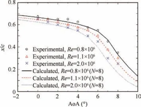
Fig. 4 Comparison of experimental and calculated result on transition position.

(2) VITA analysis

The Markov process was expected to be used to describe the fluctuating pressure, and then a feature vector consisting of one-step transition matrix and its stationary distribution could be extracted. Therefore, it is very important to obtain the Markov state space. And the VITA method was convenient to transform the fluctuating pressure into the state space.

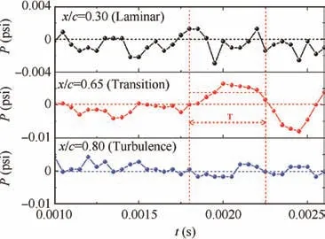
Fig. 5 Result of VITA method.

Fig. 6 Detection function of VITA method.

The result of VITA method is shown in Fig.5.The laminar and turbulent flows had stronger fluctuating feature compared to transition in the average time interval T,while the fluctuating pressure amplitude in transition zone was significantly larger in the whole time, which can be seen from Fig. 2. Such fluctuating pressure characteristics made the transition zone be more pronouncedly intermittent. And the difference of the fluctuating feature in transition, laminar and turbulent flows made the different performance in the detection function in Eq. (2), as shown in Fig. 6.

The detection function calculated by the VITA method with the parameters of K=1.0 and T=0.00025 s of the fluctuating pressure presented in Fig. 2 is shown in Fig. 6. The detection function of the transition position was significantly different from the laminar and turbulent flows whose detection function of the transition zone was mostly D=0. The VITA method essentially played the role of low-pass filtering. And the effects of parameters K and T will be discussed in detail in Section 4.1.

The number Ndof the data whose detection function is D=1 in Fig. 6 was calculated, and the cumulative time Δt=Nd/ fswas calculated as shown in Fig. 7.

The comparison of the fluctuating pressure RMS value with the cumulative time Δt calculated by the VITA method is shown in Fig. 7, where the hollow circle is the dimensionless RMS result and the solid square is the cumulative time. The minimum cumulative time position corresponded to the RMS peak position which was consistent with the research results.14,15

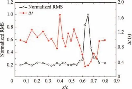
Fig. 7 Comparison of RMS and VITA results.

3.2. Establishment of Markov chain model

The fluctuating pressure data in the case of Re=1.1×106and α=2°was still taken as an example to obtain the Markov chain.

The VITA (K=1.0, T=0.00025 s) results at x/c=0.65(transition) position in Fig. 6 were analyzed. Its transition probability matrix was given as.

In fact, the sampling time Tswas used to normalize the cumulative time Δt in the VITA results through Δτ=Δt /Ts, which was essentially the calculated method of the steady-state distribution π2. Hence, the cumulative time of the VITA analysis results of the fluctuating pressure data was essentially the steady-state distribution of its Markov chain.

The feature attributes of all hidden attributes (transition and non-transition)in the sample data were averaged and were used as a stationary distribution of the observable state in the hidden Markov model.

3.3. Solution of HMM

The experimental data in the case of Re=1.1×106was used to solve the HMM.The parameters of K and T were still set to K=1.0 and T=0.00025 s.

In the solution process of the least quadratic problem which could be seen in Section 2.4 for detail, the parameters were selected as shown in Table 1.In the table,m represents m hidden attributes. There were two hidden attributes which weretransition and non-transition in this article, so m was taken as m=2.

Table 1 Parameters in the least quadratic problem.

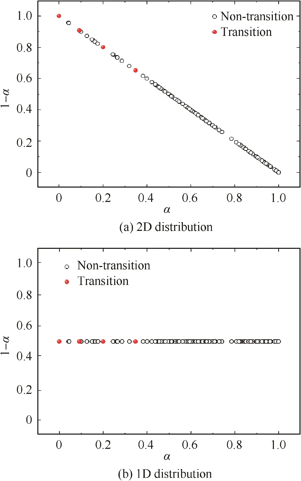
Fig. 8 Distribution of hidden attributes (K=1.0).

The smooth distribution of hidden attributes was solved using the methods in Sections 2.3 and 2.4 as shown in Fig. 8(a). Since there were only two hidden attributes, the distribution can also be described as shown in Fig. 8(b).

As can be seen from Fig.8,the distribution of the two hidden attributes(transition and non-transition)overlaps in some areas, which results in unclear classification boundaries. And we will propose a classification model with probability interpretation in order to solve this situation in the following section.

3.4. Establishment and evaluation of classification model

Considering the distribution of Fig. 8, we believe that the two hidden attributes were subject to different probability density distributions. Let’s assumed that it follows a Gaussian distribution within the interval [0,1], and the probability outside the interval is zero, which is.where μ0is the mean value,σ is the standard deviation,and c0is a constant satisfying∫∞

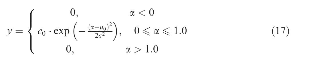
Fig. 9 Probability density distribution of transition and nontransition.

-∞ydα=1, that is.

where β1and β2are the β values of transition and nontransition respectively; P1and P2are the probabilities of transition and non-transition respectively.

Using the above method,the probabilities of transition corresponding to different α values could be calculated. The classification boundary is presented as shown in Fig. 10.

Fig. 10 Classification boundary.

For the classification model as shown in Fig. 10, the crossvalidation method was used for evaluation.The problem studied in this study was a binary classification problem, so a 2D confusion matrix was used, as shown in Table 2, where TP is the true positives,FP is the false positives,FN is the false negatives, and TN is the true negatives.

The following four indicators were used to evaluate the proposed classification model in this paper:

In general, as these indicators gradually increased, the model evaluation capability gradually enhanced.

Researchers can get a clearer understanding of the entire building process of the developed model in this article through the flowchart in Fig. 11.

4. Results and discussion

The experimental data with the Reynolds number of Re=1.1×106at AoA=0° - 7° were used to train and cross-validate the model in this section. The effects of the parameters T and K on the classification model were discussed.The prediction results of the train data (Re=1.1×106) were presented and the generalized results of other Reynolds numbers were also presented.In addition,we performed a deep theoretical analysis on the developed model, and discussed the effects of the parameters μ and σ on the classification boundary.

4.1. Parameter effects

In the building process of the developed model, there are two parameters that need to be confirmed in advance,which are T and K.The two parameters play an important role in the transformation of time series to state space.

For T,it can be seen from Section 3.1 that the parameter T essentially corresponds to the cutoff frequency of the VITA method. Therefore, the feature frequency at the transition position was first examined in order to avoid filtering out the transition features.

The power spectrums corresponding to Fig.2 are shown in Fig. 12. The frequency domain performance of fluctuating pressure at the transition position was also significantly different from that in the laminar and turbulent flows, which was that the transition region had a distinct broadband energy distribution.

The power spectrums at transition positions in the case of Re=1.1×106are shown in Fig. 13. The transition position moved forward and the characteristic frequency gradually increased when the AoA gradually increased.

Table 2 2D confusion matrix.

Fig. 11 Construction framework of developed mode.

Fig. 12 Power spectrums at typical positions with AoA=2°.

Fig. 14 Classification boundaries at different K values.

Fig. 13 Power spectrums at transition positions.

In order to cover the characteristic frequency of transition,the cutoff frequency was taken as f=4000 Hz.Therefore, the parameter T was taken as T=1/f=0.00025 s to ensure the effectiveness of the VITA method. And this was also the reason why the parameter T was selected as T=0.00025 s in Section 3.1.

The effect of parameter K on classification results was also studied.The classification boundary curves at different parameter K values are presented in Fig.14.In the actual application process, the K value of the data to be predicted is consistent with the K value in Fig.14.To assess the effect of the K value,the model was evaluated using the method in Section 3.4.Four rounds of cross-validation were performed on the experimental data, and the average value of the indicators was taken as the final evaluation index of the model.

Tables 3-5 are the evaluation results under different K values. The developed model possessed high accuracy and recall rate, and the precision was slightly lower, but it was acceptable.

The final evaluation results in Tables 3-5 are shown in Fig.15.The K value had little effect on the classification ability of the developed model. Therefore, the parameter K was selected as K=0.6 in this paper.

4.2. Prediction results of training data

Model training and prediction were performed using the experimental data of Re=1.1×106, and the model parameters were selected as f=4000 Hz, K=0.6 as discussed in Section 4.1.

Fig. 16 is a prediction result of the training data itself(Re=1.1×106). The hollow circle is a normalized RMS result, and the filled circle is the predicted property of transition using the developed model. One ‘‘transition point” could only be judged by using the RMS criterion,while a reasonable‘‘transition zone” defined as the property of transition greater than 0.5 could be obtained by using the developed method.The transition point judged by the traditional criterion was located at the transition zone. To some extent, the reliability of the two methods was demonstrated.

In this paper,the traditional RMS criterion is used to mark the data.As shown in Fig.16,only one transition position can be marked for each AoA.When using the developed model forprediction,it is possible to predict multiple transition positions at one AoA,which leads to a larger number of FP in the confusion matrix and a lower precision of the model P as shown in Fig. 15.

Table 3 Evaluation results at K=0.6.

Table 4 Evaluation results at K=0.8.

Table 5 Evaluation results at K=1.0.

Fig. 15 Evaluation results under different K values.

In order to further verify the rationality of the transition zone obtained by the developed model, the CFD method was used to calculate the transition position. The outer field was 100c, 260 grid nodes were arranged on the airfoil surface,and the height of the first layer was h/c=3×105. The global and local grids are shown in Fig.17.The COUPLE algorithm was used to solve the Reynolds Averaged Navier-Stokes(RANS) equation, and the transition SST model was selected as the turbulence model. The cases of AoA=1° and AoA=2°for Re=1.1×106were calculated.After the calculation converged, y+≈1.0.

Fig. 16 Judgement results of training data itself (K=0.6,Re=1.1×106).

Fig.18 is a comparison between the prediction results of the model developed in this paper and the CFD results.The black solid line and the red dashed line represent the transition probability results predicted by the model and the surface friction coefficient Cfcalculated by CFD, respectively. At the two AoAs, the area where the transition probability was greater than 0.5 was in good agreement with the area where the surface friction coefficient increased, which further verified the effectiveness of the developed model.

Compared with the RMS criterion, the developed model could obtain the probability that the measurement point position was transition without comparison of multi-point data.And it could obtain a reasonable and credible transition zone.This is an important advancement in transition detection using fluctuating pressure in wind tunnel experiments,and it can also provide new ideas for other transition detection methods and transition detection in flight experiments.

In fact,the construction framework proposed in this article may be not limited to the fluctuating pressure data,but be also applicable to hot-wire data. There are different transition mechanisms in different experimental conditions,different airfoil types,and even other models(flat plates,large aspect ratio wings, rear wing, hypersonic aircraft precursors, etc.), including Tollmien-Schlichting (T-S) wave transition, cross flow transition, etc. For different transition mechanisms, the

Fig. 17 Computed mesh.

It can be seen from Fig.16,Fig.19 and Fig.20 that we can predict the transition under different Reynolds numbers using the experimental data of the same Reynolds number for model training, which indicated that the developed classification model possessed strong generalization ability. Compared with the traditional RMS criterion, a reasonable transition zone corresponding to a transition point determined by the RMS criterion could be obtained by using the developed prediction model.

The comparison between the results of this paper and the traditional RMS results is shown in Fig. 21, in which the shadow part is the transition zone calculated by the developed model, the black solid line is the mean value of the shadow part, and the red dotted line is the RMS result.

For the conventional RMS criterion,the transition position moved forward with the increase of the Reynolds number in the general trend. However, the transition position did not change with the Reynolds number in the case of Re=0.8×106and Re=1.1×106, which was caused by the insufficient spatial resolution of the sensor arrangement.In addition, the transition positions of AoA=1° and AoA=2° did not change with the AoA in the case of Re=0.8×106and Re=1.1×106, which was also caused by insufficient spatial resolution of the sensor arrangement.

For the developed model, it could predict a reasonable transition zone which was different from the traditional RMS criterion. With the increase of Reynolds number, the transition zone gradually moved forward, and the transition zone gradually decreased. As the AoA gradually increased,the transition zone gradually moved forward, which was consistent with the general law of transition. It solves the deficiency of the traditional RMS criterion to some extent.

4.4. Further discussion of developed model

extracted features are different when performing ‘‘Feature extraction”in Fig.11,which will lead to different specific classification models.However,the model construction framework proposed in this article is still effective. Reflected in specific issues, there will be differences in the ‘‘Fluctuating pressure data” and ‘‘Feature extraction” links in Fig. 11.

4.3. Generalization results of other Reynolds numbers

The model trained in Section 4.2 was generalized to the case of Re=0.8×106and Re=2.0×106in this section.

Fig. 19 and Fig. 20 are the generalization results of Re=0.8×106and Re=2.0×106respectively. The hollow circle is a dimensionless RMS result, and the filled circle is the predicted result of the model.Same as in Fig.16,one transition point could only be judged using the traditional RMS criterion,while a reasonable transition zone could be obtained by using the developed model.

The developed model was based on the Markov state space which was transformed by the VITA method. The cutoff frequency of the VITA method was determined according to the characteristic frequency of transition. Within the scope of this paper, the cutoff frequency of the VITA method covered the characteristic frequencies of all Reynolds numbers,so the developed model could be effectively and reliably classified.We established a binary classification model with probability interpretation which can be seen from Fig. 9. For this classification model,a theoretical analysis on its recall rate and accuracy was performed.

The schematic diagram of the binary classification model is shown in Fig. 22, where A is a positive event and B is a negative event. Reflected in this article, event A is transition and event B is non-transition. It may be assumed that these two events are subject to the following Gauss distribution:

Under such description,the probability 1-P(B|A)=1-S3is the recall rate in Section 3.4. It can be seen that for the binary classification model in Fig. 9, the theoretical recall rate is Recall=1-S3=0.8956, and the calculated recall rate in Section 4.1 (K=1.0) is Recall=0.8750, which is consistent with the theoretical results.

Fig. 18 Comparison of judgement results using developed method and CFD results (K=0.6, Re=1.1×106).

Fig. 19 Generalization results (K=0.6, Re=0.8×106).

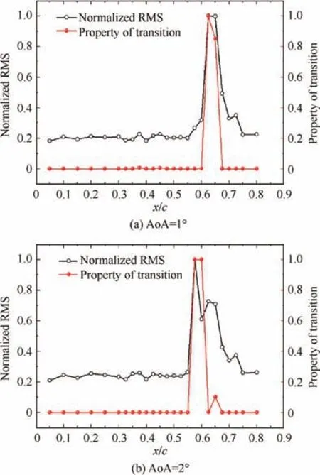
Fig. 20 Generalization results (K=0.6, Re=2.0×106).

Fig. 21 Effect of Reynolds number on transition results.

Fig. 22 Schematic diagram of binary classification model.

Table 6 Effect of parameter K on μ0 and σ.

For P(AB), it is described in the theory of probability that events A and B occur at the same time which is reflected in this article, that is, transition and non-transition occur simultaneously,which is obviously not practical.In fact,this just reflects the insufficient classification ability of the model, that is,region S3is located where the model classification is not accurate.Thus,the theoretical accuracy of the model in Section 3.4 can be calculated by.

It can be seen from Eq. (23) and Recall=1-S3that the smaller the cross region S3is, the better the classification ability of the model will be.For the model shown in Fig.9,the theoretical accuracy is 0.9449, and the accuracy calculated in Section 4.1 (K=1.0) is 0.9133, which is consistent with the theoretical results.

In fact, the parameter K affects μ0and σ of two events(transition and non-transition) as shown in Table 6, which affects the model morphology in Fig. 9. And the cross region S3is also affected by the parameter K. Then, the theoretical recall rate and accuracy can be calculated according to the above.

For the model shown in Fig. 9, the theoretical recall and accuracy under different threshold K were calculated using the parameters in Table 6, as shown in Fig. 23.

As K gradually increases, the theoretical values of both recall and accuracy gradually decrease,which is the deeper reason why K=0.6 was finally selected in Section 4.1.

On the other hand, the intersection area S3also affects the shape of the classification boundary,and S3is directly affected by μ0and σ in the Gauss distribution. Next, the effects of μ0and σ of the two Gauss distributions will be discussed.

σ was first fixed as σ=0.15,and the effect of the μ0on the classification boundary was studied by changing Δμ in Fig.24.

Fig. 23 Theoretical values under different K values.

Fig. 24 Effect of Δμ on classification boundary.

The effect of Δμ on the classification boundary is shown in Fig.24.For the classification boundary in Fig.24(b),the maximum slope was calculated as shown in Fig.24(a).The effect of Δμ on the classification boundary |k| was linear.

For the classification curve shown in Fig. 24, while changing Δμ, μ1+μ2=1.0 was ensured. However, in practical engineering applications, it generally does not satisfy μ1+μ2=1.0 (see Table 6). It is easy to think that for the Gauss distribution of σ1=σ2,when μ1+μ2changes,the classification boundary shown in Fig.24(b)shifts,and its center is(μ1+μ2)/2.

σ also has a significant effect on the shape of the classification boundary. The effect of σ on the classification boundary was studied. Here, Δμ is fixed as Δμ=0.6 and let σ1=σ2.

Fig. 25 Effect of σ on classification boundary.

The effect of σ on the classification boundary in the case of σ1=σ2is shown in Fig.25.The effect of σ on the classification boundary |k| was obviously non-linear. When σ was small, |k|increased significantly, making the classification boundary in Fig.25(b)closer to the step function.The classification boundary was more sensitive to the changes of σ compared with μ0.

However, in practical engineering applications, σ1and σ2are not equal in most cases(see Table 6).The effect of different σ combinations on the classification boundary was studied in the case of σ1=0.1 as shown in Fig. 26, and σ2is changed by changing σ2/σ1.

The effect of σ2/σ1on the classification boundary was also nonlinear.In Fig.26(b),the red circle is the maximum|k|position, and the red dotted line is the 4th-order fitting result. It could be seen that σ2/σ1would also change the shape of the classification boundary. The entire classification boundary shifted, and the classification boundary was also distorted,which showed that the classification ability was no longer 0.5 at the maximum |k| position. When σ2/σ1＞1, the property at the maximum |k| position was less than 0.5, while when σ2/σ1＜1,the property at the maximum|k|position was larger than 0.5.It could be seen that σ had an important effect on the shape of the classification boundary.

In an ideal situation,when S3=0,that is,there is no intersection area of the two probability density distribution functions in Fig. 22, the recall and accuracy of the model are all 100%according to Eq.(22)and Eq.(23),and the classification ability is the strongest.At this time,the classification boundary will take the form of a step function,and its maximum|k|will be +∞. In fact, it is impossible to achieve such an ideal situation, and we can only adjust K as much as possible to make the classification boundary approach a step function,as shown in Fig. 14.

5. Conclusions

Fig. 26 Effect of σ2/σ1 on classification boundary.

In this paper, a supervised learning model with probability interpretation for transition judgment based on experimental data was developed.It was verified by cross-validation method that the accuracy and recall rate of the model were high, indicating that the model was reliable and effective.

(1) Compared with the traditional RMS criterion,a reasonable transition zone could be obtained by using the developed classification model and it did not require comparison of signals measured at multiple locations.

(2) The effects of parameters T and K in the model were studied. The parameter T essentially affected the cutoff frequency of the VITA method. In order to not filter out the transition information, the cutoff frequency was set to f=4000 Hz, so the parameter T was T=1/f=0.00025 s. And the parameter K had little effect on the classification ability of the developed model.

(3) The generalization ability of the developed model was verified by the results at different Reynolds numbers,and the results show that the model possessed strong generalization ability.

(4) An in-depth theoretical analysis of the model was performed and the results showed that the parameters μ0and σ in the Gauss distribution affected the recall rate and accuracy in theory and they also affected the shape of classification boundary of the model.

The developed supervised learning model is an important advancement in transition detection based on fluctuating pressure, and it also provides new ideas for other transition detection methods and transition detection in flight experiments.Furthermore, this paper may propose a universal supervised learning model with probability interpretation construction framework for transition judgment, which is not limited to fluctuating pressure data and specific transition mechanism.

Declaration of Competing Interest

The authors declare that they have no known competing financial interests or personal relationships that could have appeared to influence the work reported in this paper.

Acknowledgements

The authors acknowledge all the experimental staff of NF-3 wind tunnel for their hard work. This study was supported by the National Key Laboratory of Science and Technology on Aerodynamic Design and Research Foundation, China.