Mechanism of Regional Subseasonal Precipitation in the Strongest and Weakest East Asian Summer Monsoon Subseasonal Variation Years

HU Haibo , DENG Yuheng FANG Jiabei and WANG Rongrong

1)CMA-NJU Joint Laboratory for Climate Prediction Studies, Instituted for Climate and Global Change Research,School of Atmospheric Science, Nanjing University, Nanjing 210093, China

2)Key Laboratory of Meteorological Disaster of Ministry of Education, Nanjing University of Information Science and Technology, Nanjing 210044, China

Abstract Using the National Center for Environment Prediction Climate Forecast System Reanalysis coupled dataset during 1979– 2010, we selected four subseasonal indexes from the 16 East Asian Summer Monsoon (EASM)indexes to characterize the subseasonal variability of the entire EASM system. The strongest (1996)and weakest (1998)years of the subseasonal variation were revealed based on these subseasonal EASM indexes. Furthermore, three rainfall concentration areas were defined in East Asia, and these areas were dissected by the atmospheric midlatitude jet stream axis and the position of the Western North Pacific Subtropical High (WNPSH). Then, the subseasonal effects of the WNPSH, the South Asian High (SAH), the Mongolian Cyclone (MC), and the Boreal Summer Intraseasonal Oscillation (BSISO)on each rainfall concentration area were studied in the strongest and weakest subseasonal variation years of the EASM. During the summer of 1998, the WNPSH and the SAH were stable in the more southern region, which not only blocked the northward progression of the BSISO but also caused the MC to advance southward. Therefore, the summer of 1998 was the weakest subseasonal variability of the EASM, but with significant subseasonal precipitation episodes in the northern and central rainfall areas. However, in 1996, the BSISO repeatedly spread northward in the south rainfall area because of the weak intensities and northern positions of the WNPSH and the SAH, which caused significant subseasonal precipitation episodes. In addition, MC was blocked to the north of approximately 42˚N with a weak subseasonal rainfall.

Key words East Asian Summer Monsoon; Subseasonal; Western North Pacific Subtropical High; Mongolian Cyclone; Boreal

1 Introduction

The East Asian Summer Monsoon (EASM)is the main atmospheric circulation system affecting the summer atmospheric circulation (Chen and Chang, 1980; Wang and Li, 1982; Tao and Chen, 1987; Kanget al., 2002). It can cause significant precipitation in China, which is benefits the development of China’s economy and agriculture. However, the abnormal interannual changes in the summer rainfall, such as droughts and floods caused by changes in the strength of the EASM, considerably affect people’s lives and property safety. Therefore, understanding the variations in the EASM is important.

The research regarding the EASM can be traced back to the study conducted by Prof. Kezhen Zhu on the possible effect of the EASM precipitation in China (Chu, 1934).Since the 1980s, scholars have systematically expounded the formation and characteristics of EASM winds from large-scale mean circulation, the heat source of the EASM,the early phase of the EASM-‘Mei-Yu’ regime, the transitions of the EASM, and other aspects (Lau and Li, 1984).Since then, the understanding of the EASM has gradually deepened. The EASM has significant interdecadal, interannual, seasonal, and subseasonal variations. On the interdecadal scale, the intensity of the EASM has a significant trend (Zenget al., 2007). The intensity of the EASM has periodic oscillations of 2, 4, and 7 years on the interannual timescale (Dinget al., 2013). Accompanied with the tropospheric quasi-biennial oscillation, the summer precipitation over East Asia also has obvious quasi-biennial characteristics (Meehl and Arblaster, 2001)probably because the quasi-biennial oscillation of tropical western Pacific heating can greatly affect the EASM and the water vapor transport driven by it (Huanget al., 2006). Furthermore, several studies defined an interannual monsoon index to evaluate the interannual intensity of the EASM and establish the variation law of monsoon intensity. Guo(1983)defined the atmospheric pressure gradient between the land and sea, considering the relationship between the generation of monsoon phenomenon and the land-sea distributions. Then, Shi revised another interannual index to reflect the intensity of the EASM (Shiet al., 1996). Wanget al.(2008)collected the existing 25 interannual EASM indexes and proved a good consistency on the interannual EASM strengths. Furthermore, from the perspective of interannual variabilities, changes in the Western North Pacific Subtropical High (WNPSH)are closely related to those in the EASM (Liet al., 2017). Aside from the WNPSH, the South Asian High (SAH)also affects the amount of precipitation in the Yangtze River Basin (Weiet al., 2015).Moreover, the interannual variation of rainfall in Northeast China is related to the Northeast China cold vortex(NECV)in early summer, which is mainly affected by the interaction between the WNPSH and the NECV in late summer (Shenet al., 2011). Furthermore, many works have documented the interannual influences of sea surface temperature anomalies in the Indian Ocean and tropical Pacific, including the ENSO events, the Indian Ocean Dipole, and the Indian Ocean Basin modes, on the EASM(Yuanet al., 2008).

From the seasonal perspective of the EASM, many studies have shown that the spring precipitation in South China is earlier than that in the EASM. The rainfall in the south of the Yangtze River began in early April. Then, the South China Sea summer monsoon broke out and pushed northward, which was believed as the prelude to the outbreak of the EASM (Zhuet al., 2011; Zhu and He, 2013;Zhu and Li, 2017). The South China Sea summer monsoon outbreak was probably caused by the enhanced SAH that penetrated deeply into the South China Sea around the 27th pentad (Zhuet al., 2012; Liu and Zhu, 2016). The land-sea thermal contrast participates in the formation and maintenance of the EASM, including the influence of the seasonal transition of land-sea thermal contrast and the influence of the Tibet Plateau (He and Liu, 2016). The movement of the rain belt is significantly related to the EASM.To divide rainfall regions, previous studies used statistical methods to classify the years into different rainfall distribution characteristics, namely, northern, intermediate, and southern types (Liaoet al., 1981). Some researchers proposed a detailed classification method, dividing Chinese rain areas into four or six regions from the perspectives of forecast, climate, and causes (Sunet al., 2005).

In addition to the above seasonal to interannual changes,significant subseasonal oscillations also occur in the EASM(Lau and Li, 1984). As early as the 1970s, studies provided a relatively complete explanation of the subseasonal oscillation of the EASM. They believed that the oscillation is correlated with the quasi-biweekly oscillation of the Indian monsoon system, including the Tibetan Plateau high pressure and the trans-equatorial low-level jet (Lau and Li,1984). Further research showed that the summer subseasonal precipitation in mainland China has an oscillating period of 20 – 40 d (Lauet al., 1988). In the climatic sense,the convection and wind field of the EASM also have stable subseasonal oscillation, which takes approximately 20 – 70 d (Wang and Xu, 1997). Recent studies have found that the subseasonal oscillation of the EASM in the sense of climate takes 40 – 80 d. The circulation structure shows the gear coupling mode of the WNPSH, the SAH, and the MC. When the three circulations are strengthened uniformly, the circulations lead to a three-pole distribution of rainfall in East Asia. When the WNPSH and the MC are strengthened and the SAH is weakened, a dipole distribution of rainfall occurs in East Asia (Songet al., 2016).Guanet al.(2019)revealed that the westward extension and eastward retreat of the WNPSH change the subseasonal rainfall over East Asia, and the reasons for the subseasonal oscillation of the WNPSH are different in early and late summers. In addition to the circulation factors mentioned above, the BSISO acts as an extension of intraseasonal oscillation (ISO)and plays an important role in the circulation of subseasonal EASM, including the establishment and outbreak of the EASM (Moonet al.,2013). Therefore, the WNPSH, the SAH, the MC, and the BSISO all significantly influence the variations in the EASM, including the subseasonal to interannual timescales.Considering the coupling of three impact factors, the circulation of the EASM is different (Songet al., 2016). However, on the subseasonal timescale, the possible relationships between the BSISO and the WNPSH, the SAH and the MC remain unclear.

Given the above background, many scholars have studied the interannual intensity of the EASM by defining the interannual index. However, whether or not these numerous interannual EASM indexes can be directly applied to the subseasonal time scale has yet to be determined. At this point, on the subseasonal scale, whether or not these indexes have the same synchronicity as when revealing the interannual strength of the EASM must be identified. In the presence of a subseasonal EASM index, the strongest and weakest years of the changes in the EASM on the subseasonal time scale under the definition of this subseasonal index need to be revealed. The different regions must be characterized considering the complex regional performances of summer precipitation in East Asia and the many potential influencing factors. On the basis of the above issues, this paper is outlined as follows. Section 2 introduces the data and selection method of subseasonal disturbance indexes. The division of rainfall concentration areas is discussed in Section 3. Section 4.1, Section 4.2, and Section 4.3 present the impacts of the WNPSH,the SAH, the BSISO, and the MC on different rainfall concentration areas, respectively.

2 Data and Methods

2.1 CFSR Dataset

The National Center for Environment Prediction Climate Forecast System Reanalysis (NCEP/CFSR)data were developed by the Center for Environmental Prediction in the United States and provided by the coupled air-sea model.They provide the highest-resolution coupled atmosphericocean reanalysis data in the world. As a relatively complete third-generation data set, the NCEP/CFSR data set has a series of advantages, including improved model, high resolution, assimilation scheme optimized several times,and atmospheric-land-sea-sea ice coupling setting. The results obtained with this data are accurate. This information was completed over a period of 32 years, from 1979 to 2010, and is constantly updated and expanded. The NCEP/CFSR is initialized four times a day (0000, 0600, 1000,and 1800). The 6-hour air-ocean analysis data and land surface data have horizontal resolutions of 0.3, 0.5, 1.0,1.9, and 2.5 degrees. The highest horizontal resolution of the atmosphere on a global scale is 0.312˚ × 0.312˚, and the vertical layer is divided into 64 layers. The highest horizontal resolution of the ocean on a global scale is 0.312˚ ×0.312˚, and the vertical layer is divided into 40 layers.The horizontal resolution of the NCEP/CFSR data used in this paper is 0.25˚ × 0.25˚, and the time dimension includes 32 years of summer (90 days, June 1 to August 29)from 1979 to 2010. The data variables from CFSR include surface precipitation, outgoing longwave radiation (OLR),Ucomponent andVcomponent wind fields in 850 hPa, 500 hPa potential height field, potential height field, andUcomponent wind field in 200 hPa.

2.2 Method

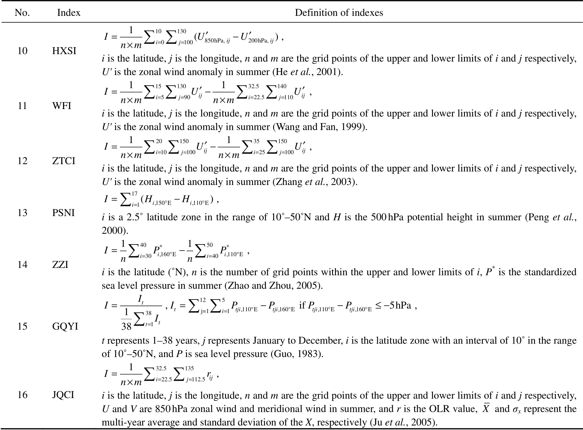
Previous studies on the EASM mostly focused on the interannual variation of the summer monsoon. More than 20 EASM indexes were defined by many researchers to describe the interannual variation of the EASM. Table 1 shows the 16 commonly used indexes to calculate and represent the variance of subseasonal disturbances.

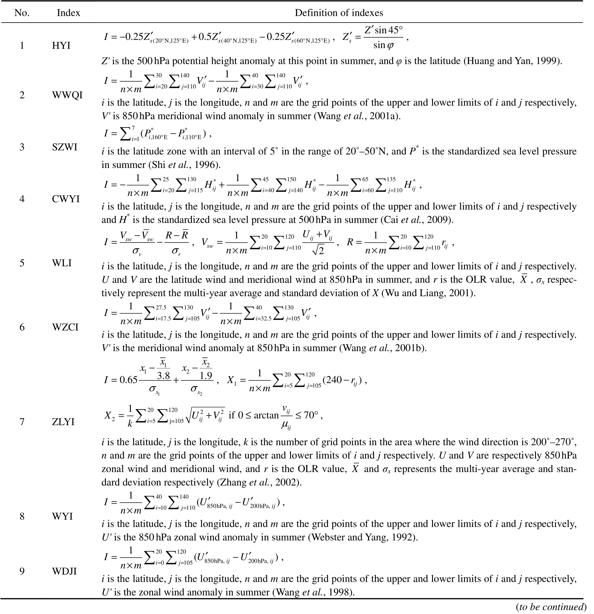
Table 1 Introduction to 16 EASM indexes

In calculating the anomaly field, the specific data of relevant meteorological elements in each year are subtractedfrom the average of last year and the seasonal evolution of the average of climate, and the moving average within ten days (hereafter referred to as a dekad,i.e., one dekad is ten days)is used to calculate the anomaly field. To simplify the steps in calculating subseasonal anomalies and obtain improved results, we adopt the definition of dekad increment to extract subseasonal anomalies (Fan and Wang, 2009).Therefore, the subseasonal disturbance variance is calculated in the present paper in the following two ways:

(continued)

1)Conventional approach: calculate the index through the daily average data of the 10-day moving average, and calculate the dekad mean value. The last 2 days (August 30– 31)of each summer (92 days)in 32 years are excluded.Then, the remaining days are divided into nine dekads for variance calculation to obtain the subseasonal disturbance variance of each year in 32 years.

2)Dekad incremental approach: calculate the mean value of dekad in each year for 92 days in 32 years, subtract the last dekad from the next dekad as the increment of dekad to obtain eight increment values every year, and then calculate the variance to obtain the subseasonal disturbance variance of the year.

The subseasonal variance values of every EASM index are calculated under the two approaches in Fig.1. The correlation coefficient between the ensembled values of the two approaches is as high as 0.75, both of which can generally describe the interannual variation of the subseasonal disturbance. However, some inconsistencies in detail are found. For example, the strongest and weakest years of disturbance under the two approaches are inconsistent because some of the 16 indexes are unsuitable for characterizing subseasonal disturbance.

To find the index representing the subseasonal disturbance of the EASM, we use the following selection criteria:the index value is calculated using the two approaches of subseasonal disturbance variance (conventional approach and dekad incremental approach). Under both approaches,the interannual variation of the disturbance variance is highly correlated with the overall average of the 16 indexes,and the strongest and weakest years are the same.

The 16 indexes and the overall average are analyzed by the Taylor diagram. On the basis of the distribution characteristics of the 16 indexes in the Taylor diagram, the index could pass the mean test when its correlation coefficient is greater than 0.4 and the standard deviation ratio is within the range of 0.5 – 2.

It indicates that the index is highly consistent with the overall average. In Fig.2, the correlation coefficients of indexes 9, 10, 11, and 12 under the conventional approach are 0.72, 0.68, 0.80, and 0.67, respectively, and the standard deviation ratios are 1.98, 1.85, 1.83, and 1.88, respectively. The correlation coefficients of these four indexes in the dekad incremental approach are 1.89, 1.77,1.53, and 0.96, and the standard deviation ratios are 0.71,0.75, 0.74, and 0.45. They can pass the test under both approaches and is highly consistent with the overall average. The correlation coefficient of the four indexes under the two approaches reaches 0.84, which can better describe the interannual variation of the subseasonal disturbance compared with the overall average of the 16 indexes. Therefore, we choose the average of indexes 9, 10,11, and 12 as the index of the change in subseasonal disturbance. The strongest annual average is 1996, and the weakest annual average is 1998. We then examine the strongest year (1996)and the weakest year (1998)of subseasonal disturbance.

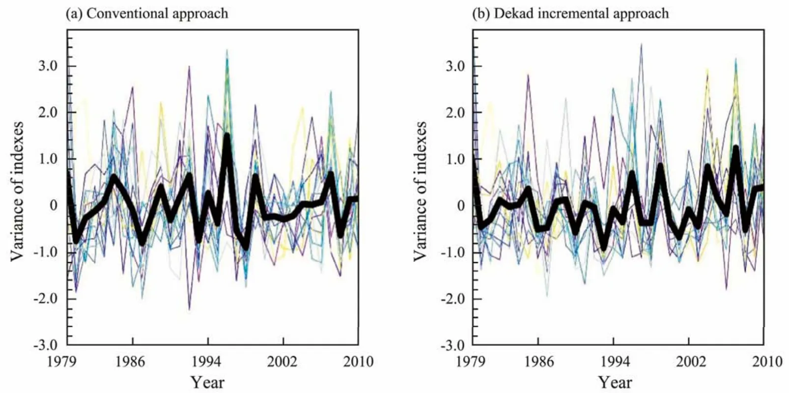
Fig.1 Interannual variation of the variance of the summer monsoon index. The 16 thin lines in (a – b)represent the (a)conventional approach and (b)dekad approach interannual variations of the 16 EASM index variances, and the black thick line represents the ensemble-mean value of 16 index variances. These indices are calculated bases on the definitions of the 16 indices given in Table 1.

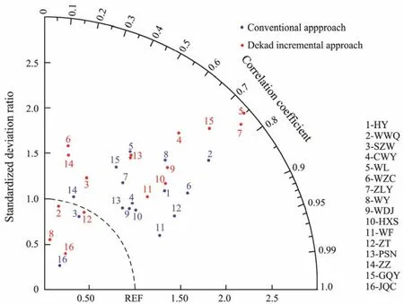
Fig.2 Taylor diagram of 16 summer monsoon indexes and their average values under two approaches. Theradius represents the standard deviation ratio is the ratio between the standard deviation of each index in 32 years and the standard deviation of the average value in 32 years under this definition. The blue solid points represent the values in the conventional approach,and the red solid points represent the values in the dekad incremental approach.

3 Definition of Rainfall Concentration Areas in the Strongest and Weakest Subseasonal Disturbance Years of the EASM

In the seasonal evolution of the EASM and precipitation,different regions have shown significant seasonal differences. To divide rainfall regions, previous studies used statistical methods to classify the years with different positions of the central main rainfall belt in China. In addition to the main rain belt, significant large-scale concentrated precipitation also occurs in other regions of China. However, few studies discussed their regional division methods. In addition, the large-scale concentrated precipitation is determined by the water vapor transport of the largescale atmospheric circulation, but the existing division of the location of the main rain belt does not directly consider the atmospheric circulation system (Liaoet al., 1981;Sunet al., 2005). As shown in Fig.3, the precipitation in eastern China can be divided into three regions according to its spatial distribution characteristics. This feature has persisted in the past 32 years. Cyclone circulation often occurs on the north side of the westerly jet, which affects the precipitation in the north of East Asia (Tao, 1980). This study proved that the location of the westerly jet plays an important role in the distribution of precipitation in the north of East Asia. Therefore, in the present study, the maximum zonal wind of 200 hPa as the jet stream axis is used as the dividing line between the rainfall in the north and south of East Asia. Moreover, the north of the ridgeline of the WNPSH contains the depression area of the WNPSH on precipitation, which can clearly separate the precipitation concentration areas into the central and southern regions. At the same time, as a dynamic barrier, it weakens or even blocks the northward subseasonal influence of the low-latitude tropical monsoon and ISO signals. Thus, it is used as the separation line between the central and southern precipitation concentration areas in this work (Wang and Ding, 2008; Zhu and He, 2013; Zhu and Li, 2017;Guanet al., 2019). Therefore, we can regard the WNPSH ridgeline as the dividing line between the precipitation in the south and the north in East Asia. In consideration of the above two atmospheric circulation factors, their location can match the precipitation concentration area very well (Fig.3).

Thus, the rainfall areas in the north of the red line in Figs.3(d – f)are called the northern rainfall concentration area (NRCA), the middle rainfall area in Figs.3(g – i)is called the central rainfall concentration area (CRCA), and the rainfall area south of the blue line in Figs.3(j – l)is called the southern rainfall concentration area (SRCA).Under the decadal average, the north margin of the CRCA is stable at approximately 40˚N, whereas the north margin of the SRCA is stable at approximately 25˚N to the east of 120˚E. However, the north margin of 100˚ – 115˚E may be affected by the SAH and thus drift southward. On the basis of the above definition of rainfall concentration area,the summer average of 1996 and 1998 is divided into three concentration areas. As shown in Fig.4, the location of the northern margin of the CRCA is in the more northern region, and the northern margin of the SRCA is generally located at 25˚ – 30˚N in 1996, which is generally more north than that of 20˚ – 25˚N in 1998. The 120˚E longitude line passing through each rainfall concentration area is taken as a profile, as shown in Fig.5. The WNPSH in 1998 is stronger than that in 1996. In addition, the distribution of three rain belts can be clearly observed. The rainfall belt in the north of the main body of the WNPSH matches well with the jet stream axis. However, significant differences exist in the rainfall zone between the two years. In 1996, this rain belt continued northward over time. In 1998, this rain belt moved with time in two processes. It spread northward from the 1st dekad to the 4th dekad and then retreated south. Then, it moved northward from the 5th dekad to the 9th dekad continuously. The rain belts located north of the jet stream axis in 2 years all spread south, but they were slightly different. In the south of 25˚N, a positive-negative transition occurred in 1996.In addition, the area of positive-negative abnormal conversion was approximately 10˚ – 25˚N, which belonged to the SRCA of 1996. Thus, we can infer factors that cause the subseasonal changes in the SRCA. However, the subseasonal changes in the SRCA in 1998 were not significant. In both years, the positive anomalous areas of precipitation underwent meridional wind convergence.

The following section of the paper explains the subseasonal changes of rainfall in each rainfall concentration area and how the external force affects these three rainfall concentrations.

4 Characteristics of External Forcing and Influence of Three External Forcing on Different Rainfall Concentration Areas

In the above definition, rainfall in East Asia has been divided into three regions. The NRCA is mainly controlled by the MC, whereas the CRCA is mainly affected by the WNPSH and the SAH. The SRCA is mainly affected by the BSISO (Shenet al., 2011; Moonet al., 2013; Songet al.,2016; Guanet al., 2019). Therefore, this paper discusses the subseasonal variation of rainfall concentration area and the influence of the corresponding forcing.

4.1 Characteristics of BSISO in 2 Years and Impact on the SRCA

The BSISO, with a periodicity of 10 – 90 days, is characterized by a pronounced northward or northwestward propagation over the East Asian and Western North Pacific (EA-WNP)regions. Meanwhile, the BSISO significantly impacts the rainfall in East Asia (Moonet al., 2013).The northward propagation of the ISO influences precipitation associated with the northward advance of the Meiyu(central China)-Baiu (Japan)front, which is related to the onset of the summer rainy season. The floods over the Yangtze River valley are mainly affected by the 30 – 60-day ISO, but the origin of the 30 – 60-day ISO is still open to question (Chenet al., 2001). From the perspective of interannual change, the variability of the BSISO mainly occurs in its evolution. The interannual variability of the BSISO propagation mode can be divided into the following four modes: northeast mode, north-only mode, east-only mode, and stationary mode. The BSISO of the northeast and north-only modes can reach the Western Pacific by passing over the Maritime Continent because of the positive mean moisture anomalies and upward mean motion anomalies over the Maritime Continent. For the east-only and stationary modes associated with the central Pacific warming, their BSISO can hardly pass the Maritime Continent because of negative mean moisture anomalies and downward mean motion anomalies (Zhanget al., 2019).Therefore, the characteristics of the propagation of the BSISO in these two years and the characteristics of the SRCA in 1996 and 1998 are discussed in the following paper.

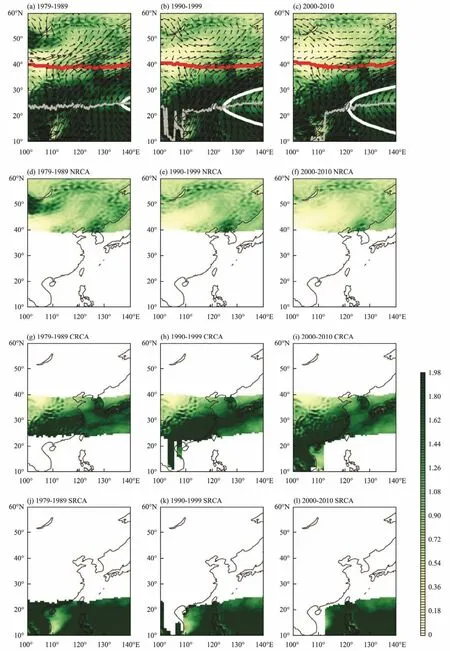
Fig.3 Division of rainfall concentration area in East Asia (10˚ – 60˚N, 100˚ – 140˚E). Shadings show the total rainfall (unit:kg m-2). The red solid line is the jet stream axis (maximum zonal wind value in 200 hPa). The 500 hPa potential height line has a value of 588 (white solid line; unit: dagpm). The gray dashed line is the maximum potential height value in 500 hPa.

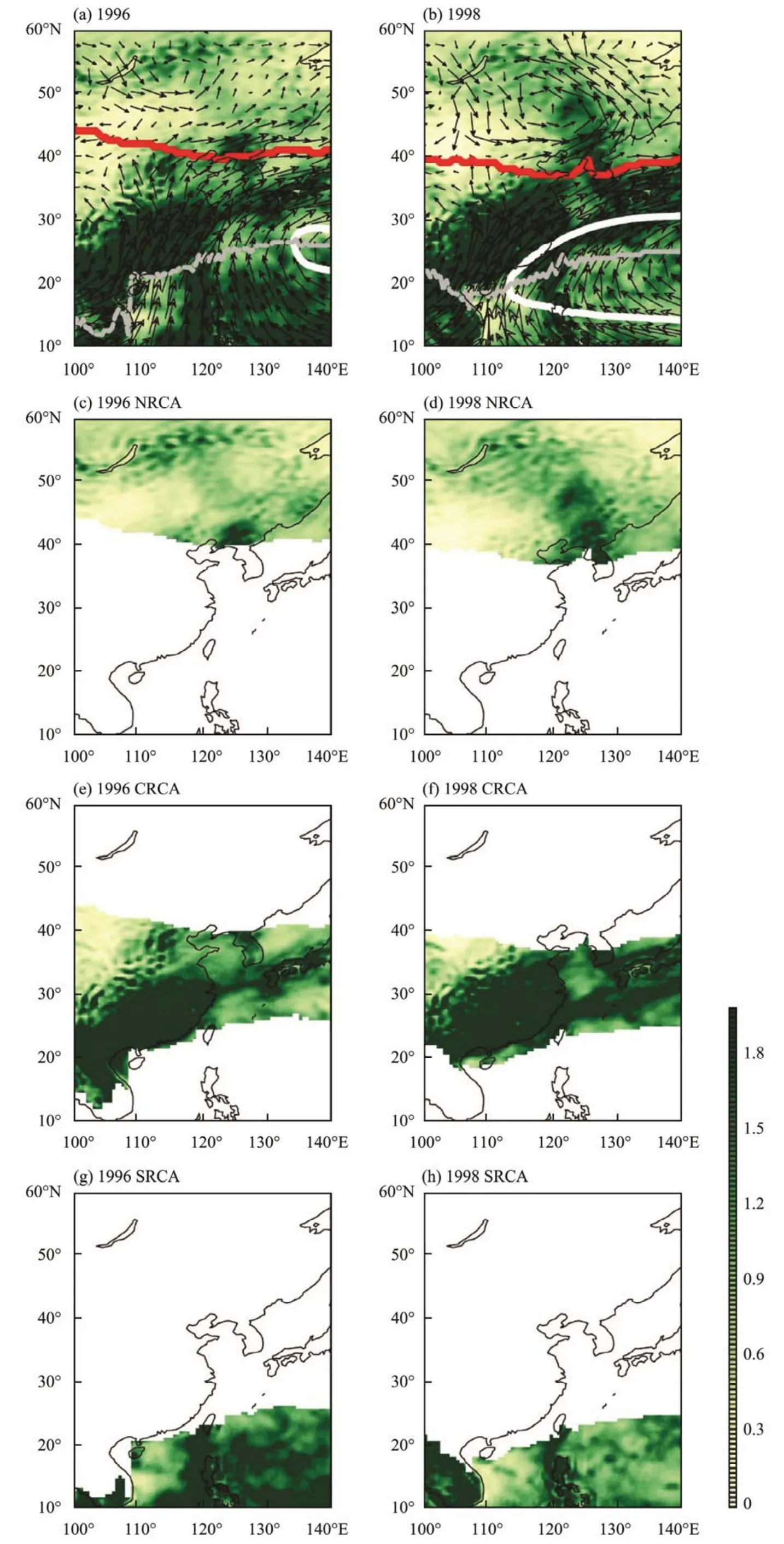
Fig.4 Division of rainfall concentration area in East Asia (10˚ – 60˚N, 100˚ – 140˚E). Shadings show the total rainfall (unit:kg m-2). The red solid line is the jet stream axis (maximum zonal wind value in 200 hPa). The 500 hPa potential height line has a value of 588 (white solid line; unit: dagpm). The gray dashed line is the maximum potential height value in 500 hPa.

Fig.5 shows the conversion of positive and negative rainfall anomalies in the 10˚–30˚N region on the nine dekads of summer, which could be the influence of the northward transmission of the BSISO. The latitude of the 120˚E profile is extended from 10˚N to 5˚N. This phenomenon allows further observation of the characteristics of time changes of the OLR in this range. As expected,the region of 5˚–10˚N has positive and negative abnormal subseasonal signals, as shown in Fig.6(a). This point is well verified in Fig.6(c). The OLR anomaly in the summer in this region shows obvious subseasonal variations of about two cycles. However, no positive and negative abnormal signal conversion was observed in 1998, as depicted in Figs.6(b)and (d). Combined with Figs.5(c–d), the BSISO signal in 1998 was blocked by the stable and strong WNPSH and SAH. The upward mean motion anomalies over the MC were restrained when the WNPSH and the SAH were steadily located farther south (Zhanget al., 2019).Thus, no signal was transmitted northward. However, in 1996, the BSISO transmitted northward because of the weak WNPSH and SAH.

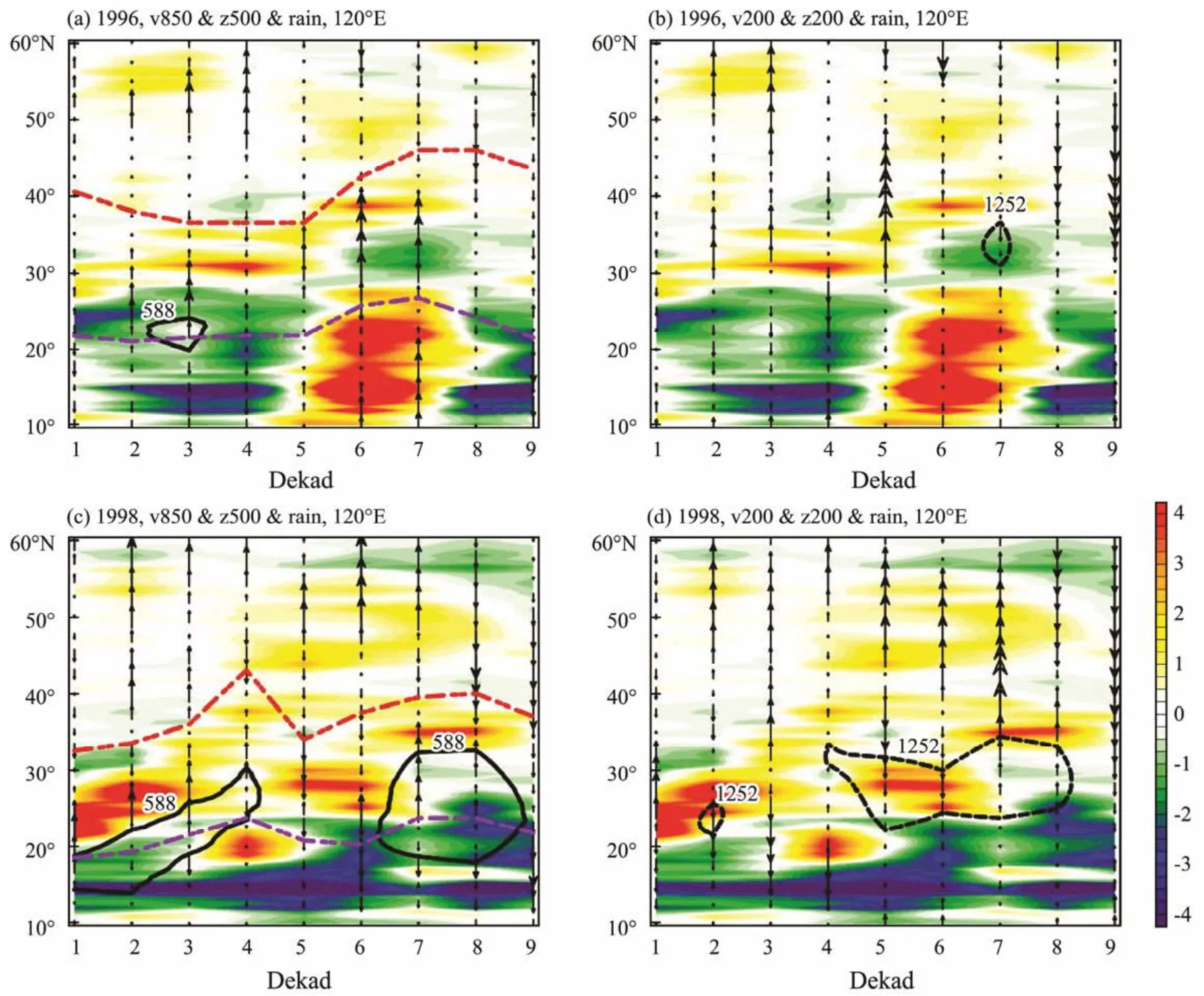
Fig.5 Precipitation anomaly, meridional wind field, and jet stream axis change with time in the 120˚N profile. (a)shows the 850-hPa meridional wind component (vector; unit: m s-1), the 500-hPa potential height line with a value of 588 (black thick solid line; unit: dagpm), the jet stream axis (red dashed line), the WNPSH ridgeline (purple dashed line), and precipitation anomaly (shadings; unit: kg m-2). (b)shows the 200-hPa wind field (vector; unit: m s-1)and the 200-hPa potential height line with a value of 1252 (black thick solid line; unit: dagpm)and precipitation anomaly (shadings; unit: kg m-2)in 1996.Similarly, results (c)and (d)show the same variables as (a)and (b)but in 1998.

Combined with Figs.5(a–b), the northward spread of the BSISO in 1996 led to the significant subseasonal variation of rainfall in the SRCA. Therefore, the subseasonal change of rainfall in SRCA was caused by the northern transmission of the BSISO, as shown in Fig.4(g). However, in 1998,the BSISO did not spread northward because of the obstruction of the WNPSH and the SAH. In addition, the rainfall in the SRCA this year showed an almost negative anomaly. Thus, the strong year of the subseasonal change corresponds to the stronger rainfall subseasonal change. In Fig.6, when the positive precipitation anomaly appears, the negative OLR anomaly also appears. The slight difference is that the occurrence time of the positive precipitation anomaly is earlier than that of the negative OLR anomaly.

4.2 Characteristics of the WNPSH and the SAH in 2 Years and Their Impact on the CRCA

The WNPSH and the SAH are opposing and facing away from the subseasonal scale, respectively (Guanet al., 2018).Their strength and the movement of northward and southward are also closely related to the MC in the north and the BSISO in the south (Songet al., 2016). In the CRCA,it is mainly controlled by the WNPSH (Guanet al., 2019).Previous studies mainly discussed the impact of the WNPSH westward extension and eastward retreat on the transportation of warm and humid airflow and abnormal precipitation in the Yangtze River Basin. The following paragraphs discuss the characteristics of the WNPSH and the SAH in the two years of the strongest and weakest subseasonal disturbances, as well as the relationship with the CRCA.

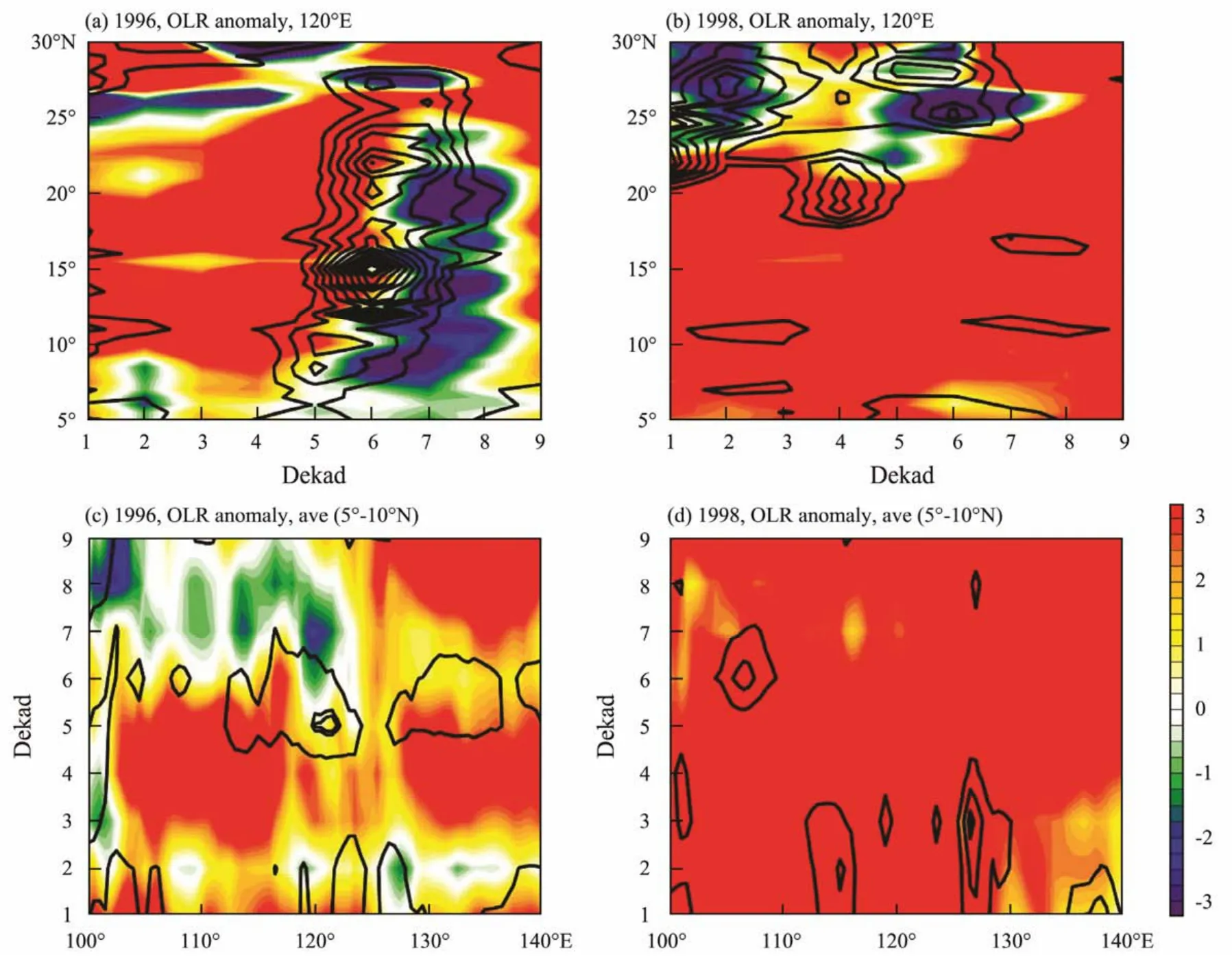
Fig.6 (a – b)120˚E profile of the OLR anomaly. The horizontal axis is nine dekads in summer. Shadings show the OLR anomaly (unit: W m-2). The black solid lines show the positive precipitation anomaly (the minimum value of contour is 0.2,and the interval is 1.2). (c – d)Profile of zonal average of 5˚ – 10˚N.

On the basis of the approximate positions of the WNPSH and the SAH in 1996 and 1998 in Fig.5, the zonal average profiles of the main bodies of the WNPSH and the SAH are shown in Fig.7. In 1996, the WNPSH appeared only for a short period of time at the average latitude, and the area was much smaller, as shown in Figs.8(a – r). In addition,the decrease in potential height of the key domain of WNPSH in Figs.8(a – r)and Fig.9(b)had a significant matching relationship with the northward movement of the WNPSH ridgeline in Figs.8(a – r)and Fig.9(a). It can also reflect the weak WNPSH intensity to some extent. The position change was also significantly different from that in 1998. In Fig.7(c), the WNPSH appeared at the 1st dekad and maintained to the 3rd dekad. In Fig.7(a), the WNPSH appeared at the 5th dekad and maintained to the 7th dekad. Thus, 1996 WNPSH had an obvious north jump process. In addition,Figs.8(a – r)and Figs.9(a – b)show that the beginning time of the north jump was roughly in the 5th dekad of the summer of 1996. Figs.7(a – d)displays that the SAH also changed with the northward movement of the WNPSH.For 1998, the WNPSH and the SAH appeared steadily in the same period with different mean latitudes. The potential height of the key domain of the WNPSH in Figs.8(a –r)and Fig.9(b)showed a downward trend with the northward shift of the WNPSH in Figs.8(a – r)and Fig.9(a).However, it was not obvious because of the strong stability of the WNPSH in 1998. Combined with Figs.8(a – r)and Figs.9(a – c), the north jump of the WNPSH in 1998 was not obvious. As illustrated in Figs.7(e – h), the difference from 1996 is that the WNPSH in 1998 had a slight northsouth oscillation in 90 days. In addition, nearly two cycles occurred in summer, accompanied by westward extension and eastward retreat. Figs.8(a – r)and Fig.9 display that the degree of the westward extension of the WNPSH in 1998 was greater than that in 1996, and its location is more to the south. Figs.8(a – r)and Fig.9 show that the west extension points of the WNPSH had the highest matching degree with the CRCA rainfall in the past two years.

For rainfall, the distribution of the rain belt had a good configuration relationship with the WNPSH. Under the control of the WNPSH, a negative anomaly of precipitation was observed. However, the SAH did not have a good configuration relationship. The difference in rainfall anomaly distribution in these two years was that the subseasonal variation of precipitation appeared further south in 1996,as displayed in Figs.7(c–d). The cycle was 90 days or so.Combined with the argument in the above section, the subseasonal variation of this rainfall may be caused by the northward transmission of the BSISO, considering that the area is roughly in the SRCA. It is not simple because of the subseasonal changes in the WNPSH. In 1998, the subseasonal changes in precipitation appeared in Figs.7(e–f)for 30–60 days (Chenet al., 2001). The subseasonal variation of precipitation in this area was mainly caused by the subseasonal change of WNPSH. Thus, the weak year of subseasonal variation corresponds to the stronger subseasonal variation of rainfall.

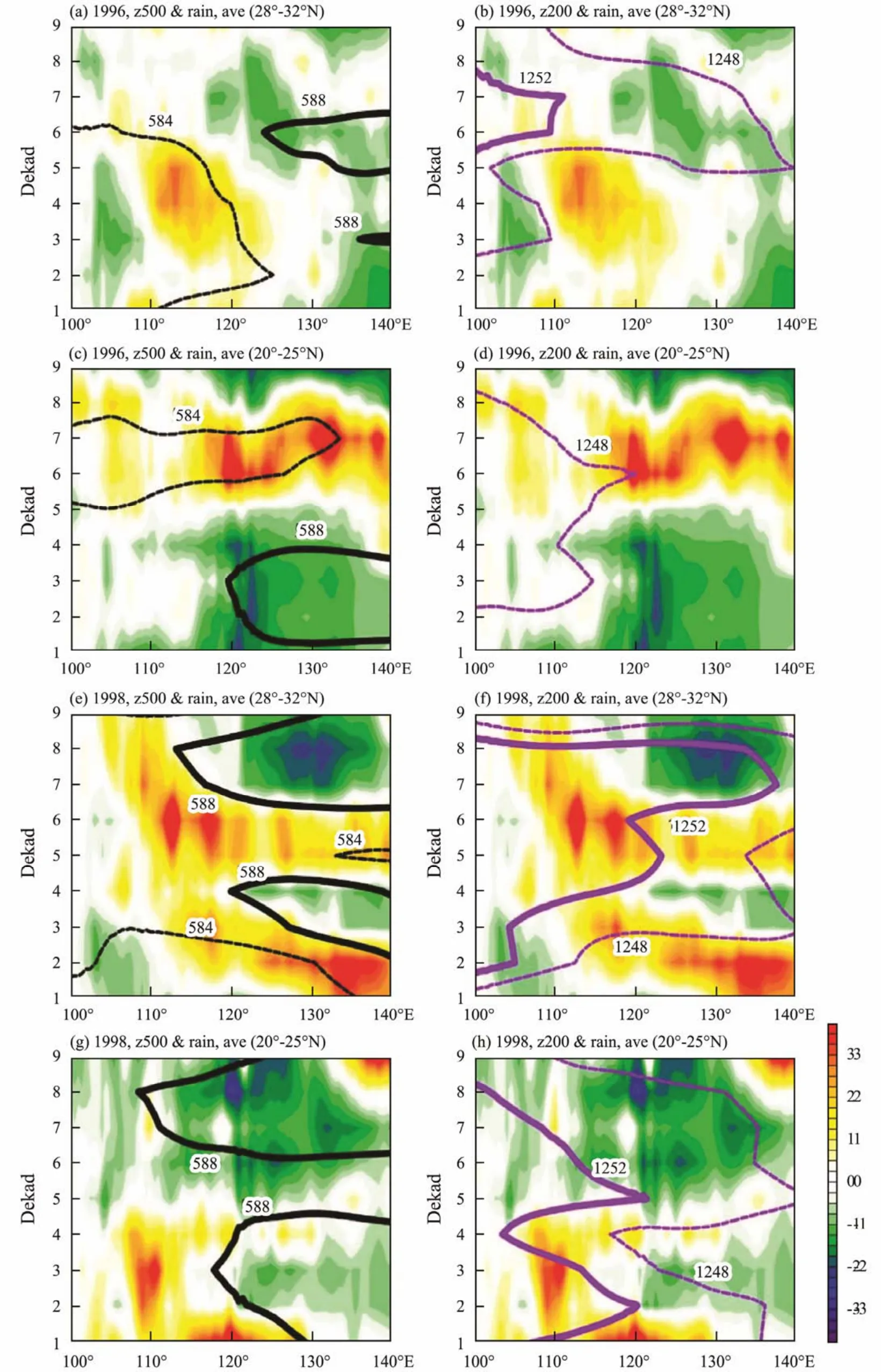
Fig.7 (a – d)Shadings show the zonal profile in 1996 (a – d)and 1998 (c – h)(unit: kg m-2). (a – b)show the main body of the SAH (zonal average of 28˚ – 32˚N). Contour lines in (a)and (c)are at 500 hPa potential height with values of 588 (black solid line; unit: dagpm)and 584 (black dashed line; unit: dagpm). (b)Contour lines in (b)and (d)are at potential height of 200 hPa with values of 1252 (purple solid line; unit: dagpm)and 1248 (purple dashed line; unit: dagpm). Similarly, (e – h)show the same variables but in 1998.

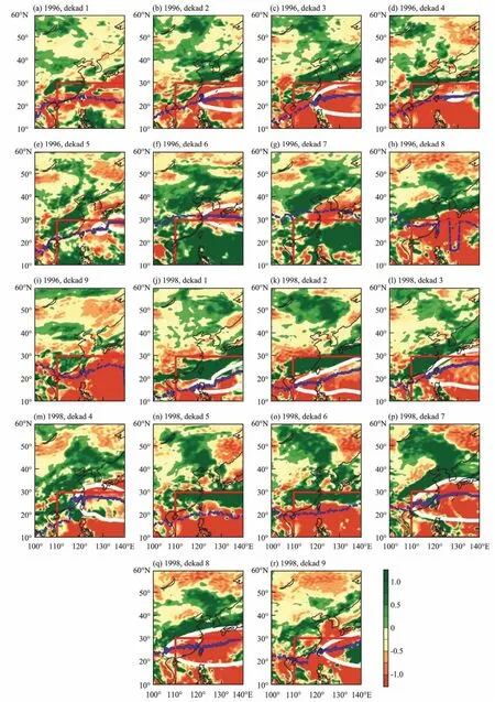
Fig.8 Evolution of the WNPSH index in the nine dekads of summer in East Asia (10˚ – 60˚N, 100˚ – 140˚E)in 1996 and 1998. Shadings show the precipitation anomaly (unit: kg m-2). The white solid line shows the 500 hPa potential height with a value of 588 (unit: dagpm). The blue solid point means the WNPSH western ridge point. The blue solid line can be used as the WNPSH ridgeline (maximum value in 500 hPa potential height), and the red box is the key domain of the WNPSH(10˚ – 30˚N, 110˚ – 140˚E). (a – i)The nine dekads of summer in 1996. (j – r)The nine dekads of summer in 1998.

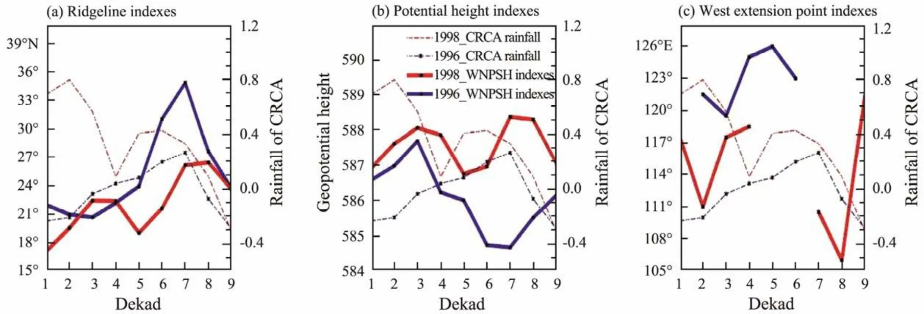
Fig.9 Variation of the three indexes of the WNPSH in summer. The WNPSH indexes in 1996 and 1998 are represented by the blue and red solid lines, respectively. The blue and red dashed lines are the variation of rainfall of the CRCA in 1996 and 1998, respectively. (a)is the WNPSH ridgeline (the horizontal axis is the nine dekads in summer;). (b)is the potential height of key domain of the WNPSH (10˚ – 30˚N, 110˚ – 140˚E). (c)is the west extension points of WNPSH.

4.3 Characteristics of the MC in 2 Years and Their Impact on the NRCA

In the 1980s, Tao (1980)proved that the MC is a circulation pattern that can result in heavy rainfall in the northeastern and northern parts of China. Many scholars then established the connection between atmospheric circulation and the MC. They further concluded that the MC was the key factor in the northern rainfall in East Asia. The rainfall caused by the MC can be divided into two rainy seasons, and the intensity of the MC also affects the abnormal rainfall (Heet al., 2007). The MC can even affect southern China (Miaoet al., 2006). However, few previous studies investigated whether or not the movement of the MC on a subseasonal scale matches the rainfall in the NRCA. Therefore, the movements of the MC and the NRCA are characterized in the present section. The impact of MC on the SRCA in the two years is also discussed.

The large value of positive vorticity anomaly can be considered as the active region of the MC. In Fig.10(a), the position of the MC in 1996 was roughly located in the 50˚– 55˚N, 105˚ – 120˚E region. This region had a large positive vorticity anomaly variance. In 1998, the position of the MC extended from northwest to southeast and formed a zonal distribution, roughly in the 40˚ – 60˚N, 105˚ – 135˚E region, as shown in Fig.10(b). The active location of the MC in 1998 was possibly wider and stronger than that in 1996, and the moving position from northwest to southeast was to the more southward region. As displayed in Figs.11(a–b), the vorticity anomaly concentration area in the south of 50˚N appeared in the 1st dekad and remained to the 3rd dekad, which is located in the west of 120˚E.The abnormal vorticity concentration area moved from north to south and from west to east, and it moved from northwest to southeast in the whole northern area of East Asia. It further proves the movement characteristics in Fig.10(a). In Figs.11(a–b), the initial occurrence time of the positive rainfall anomaly also moved from the 1st dekad of the north latitudinal mean (50˚ – 60˚N)to the 5th dekad of the south latitudinal mean (the jet stream axis to 50˚N).

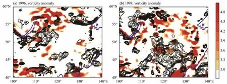
Fig.10 The variance of vorticity (shadings)and the positive vorticity anomaly (contour line; the minimum value of contour is 0.4, the maximum value of contour is 2, and the interval is 1.2)are shown in 1996 and 1998. The blue solid line indicates the terrain.

The maintenance time and the moving path were generally consistent with the MC. Similarly, in Figs.11(c – d),the configuration of positive vorticity anomaly concentration area and rainfall concentration area in 1998 moved from northwest to southeast. However, different from that in 1996, the positive vorticity anomaly in 1998 maintained for a long time in the northern and southern latitudinal averages. For the northern latitudinal mean, the concentration area of positive vorticity anomaly was maintained for about the 7th dekad in Fig.11(c). For the southern latitudinal mean, the concentration area of positive vorticity anomaly maintained from the 3rd dekad to the 9th dekad,which was longer than that in 1996, as illustrated in Fig.11(d). Meanwhile, the longer maintaining time of the positive vorticity anomaly allowed the rainfall to maintain for a longer time. Moreover, subseasonal variation of the MC occurred in both years.

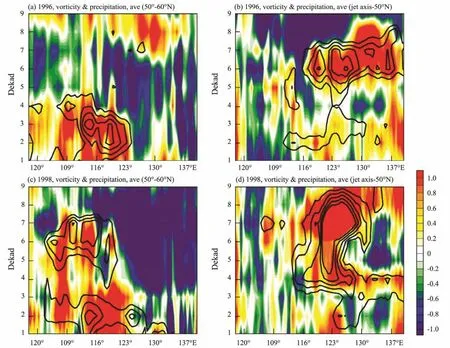
Fig.11 Shadings are the positive vorticity anomalies and the black solid lines are the positive precipitation anomalies (the minimum value of contour is 0.2, the maximum value of contour is 1, and the interval is 0.2; unit: kg m-2). Meridional averaged variables between 50˚ – 60˚N (a)and the jet stream axis to the 50˚N (b)are shown in 1996. Similarly, (c)and (d)show the same variables but in 1998.

Therefore, for these two years, the MC accompanied with the rainfall concentration area moved from northwest to southeast. At the same time, subseasonal variation of rainfall occurred in both years. However, the weak year of subseasonal variation corresponds to the stronger subseasonal variation of rainfall. When the WNPSH was in the more northern region, it weakened the MC and then made the MC move to the more northern region (Dinget al.,2019). Thus, for the weakest year of the subseasonal disturbance, the MC was stronger and moved to a more southern position. In addition, the long-term stability of the WNPSH and the MC in the northern boundary of the CRCA resulted in sustained and steady rainfall in 1998.However, it was different from that in 1996. The MC was blocked to the north of about 42˚N, which led to weaker subseasonal precipitation in the central part.

5 Conclusions and Discussion

In this paper, 16 commonly used EASM interannual indexes were selected to study their consistency and applicability on the subseasonal time scale by using the NCEP/CFSR coupled dataset during 1979 – 2010. Furthermore, two technical means were used to calculate the subseasonal variance. One was the conventional approach,and the other was the dekad incremental approach. By using ensemble-mean and Taylor diagram methods, results showed that the ensembled annual variation of the subseasonal disturbance variance of the 16 indexes has a high correlation between these two technical approaches,suggesting the generality of these two approaches in calculating the subseasonal variability. However, the 16 EASM interannual indices are not consistent in the calculation of subseasonal disturbances, although they have consistent EASM interannual variability characteristics.Among all the EASM indexes, four indexes were proven to be in good agreement with the ensemble-mean value,the ensemble-mean value of which was adopted as the subseasonal EASM index in this research. On the basis of the interannual variation of this subseasonal EASM index,the strongest (1996)and weakest (1998)years of the EASM subseasonal disturbance variance were revealed in 32 years. In addition, the significant rainfall concentration areas in the EASM seasonal process are always switching.Therefore, according to the spatial distributions of precipitation and the differences of the atmospheric circulation system, East Asia (10˚– 60˚N, 100˚–140˚E)is divided into three rainfall concentration areas in this research: the NRCA, the CRCA, and the SRCA. Then, the influences of the WNPSH, the SAH, the MC, and the BSISO on each rainfall concentration area were studied in 1996 and 1998 on the subseasonal timescale.

The CRCA is defined as the rainfall area between the WNPSH ridgeline and the jet stream axis, which is the main rain belt in summer in China. Previous studies emphasized the importance of the WNPSH and the SAH on their interannual and subseasonal variability (Weiet al.,2015; Songet al., 2016). However, our study found that the effects of the two are significantly different in different EASM subseasonal strong and weak years. In 1998,the WNPSH and the SAH were strong and stable, with a weak north–south oscillation in 90 days. In addition, the WNPSH extended to a more westward and more southward region. In 1998, the precipitation anomaly showed obvious subseasonal variation in the east of 120˚E in the zone average 28˚–32˚N, with a period of 30 – 60 d. In 1996,the WNPSH and the SAH were weak, but the WNPSH had an obvious northward jump in the 5th dekad. For CRCA rainfall in 1996, a subseasonal variation of precipitation anomaly occurred in the east of 120˚E in the zone average 20˚–25˚N for approximately 90 days. In both years, a good subseasonal relationship was found between the CRCA rainfall and the WNPSH, but no obvious relationship was observed with the SAH. The WNPSH western ridge point index had the best relationship in both years. Regardless of how strong or weak, the annual mean WNPSH was, the subseasonal variability of precipitation in this region was significant. Even in 1996, with weak WNPSH, the subseasonal variability of rainfall in the central part was stronger under our current definition (Fig.8),which is influenced by the northward jump of the south boundary of the CRCA (Fig.7). However, the northern boundary of CRCA is located to the north of 40˚N. Thus,almost no influences can be observed on the results in Fig.7.

The SRCA is defined as the south of the WNPSH ridgeline in East Asia (10˚–60˚N, 100˚–140˚E). Previous studies described the role of the BSISO in this area (Moonet al.,2013). However, our study found that the BSISO also played different roles in the two extreme summers. During 1996, the BSISO was transmitted inside the SRCA repeatedly and even spread to near 25˚N with the northward jump of WNPSH. This phenomenon made the 20˚– 25˚N region have obvious subseasonal precipitation in 1996 for approximately 90 days. However, during 1998, the BSISO could not be found in the whole SRCA region, with almost no precipitation throughout the summer in this region.Therefore, in this region, the subseasonal indexes of the EASM can indicate the intensity of the subseasonal variation of precipitation.

The NRCA is defined as the region north to the jet stream axis in East Asia (10˚–60˚N, 100˚–140˚E), which was obviously influenced by the MC on the interannual time scale (Shenet al., 2011; Tao, 1980). The subseasonal precipitation in this region was weaker in 1996 and stronger in 1998. The intensity and location of MC differed in the strong and weak years of subseasonal variability. In the year of strong subseasonal variation, the intensity of MC was weak, whose position was in the more northern region. However, for the subseasonal weak year, the MC was stronger and more stable, which could move to the more southern region. Thus, the stronger the subseasonal indexes of the EASM were, the weaker the subseasonal precipitation variability was in the NRCA.

In summary, the strong WNPSH and SAH acted like two gates, which were in the more southern position and blocked the northward propagation of BSISO in 1998.Thus, the BSISO activity and precipitation in the SRCA decreased with the weak subseasonal EASM index. The subseasonal precipitation in the SRCA region is consistent with the subseasonal variability of the EASM on the interannual time scale. However, for the CRCA, although the subseasonal monsoon index was the weakest in 1998,a significant subseasonal precipitation occurred in this region because of the strong subseasonal variable WNPSH.In the strongest year of subseasonal variation of EASM,the weaker mean intensity of the WNPSH with subseasonal variation led to the northward transmission of more BSISO signals on the southern side, which caused the significant subseasonal precipitation in the central region.The subseasonal precipitation in the central region is well correlated with the WNPSH indexes, especially the WNPSH west extension points, but not with the subseasonal EASM indexes. Finally, in the northern concentrated area, the strongest (weakest)year of the EASM subseasonal variation, accompanied by the Northern (Southern)position of the WNPSH, is unfavorable (conducive)to the continuous southward shift of MC on subseasonal time scale, which leads to the weak (strong)subseasonal precipitation in the NRCA region. The above results indicate that the WNPSH, the SAH, the MC, and the BSISO, as the main factors affecting the whole East Asian subseasonal precipitation, have different configurations in different summers, resulting in different subseasonal precipitations.The subseasonal monsoon index proposed in this paper can be used to characterize the subseasonal precipitation intensity in the SRCA, which is not applicable in the central region and has an opposite relationship in the northern region. However, the current conclusion is based on the strongest and weakest years of the EASM subseasonal variation. The results in other non-extreme strong and weak years warrant further exploration. In addition, the current analysis data use NCEP/CFSR. Whether or not this conclusion is sensitive remains to be revealed when using different data sets. Finally, the forcing factors in the observation data exist at the same time and interact with each other. We hope to improve this research by performing numerical simulations in the future, whose forcing factors can be separated.

Acknowledgements

This work was supported by the National Key Program for Developing Basic Science (Nos. 2018YFC 1505900 and 2016YFA0600303), the National Natural Science Foundation of China (Nos. 42175060, 41621005, 41675064, 4167 5067, and 41875086), the Jiangsu Province Science Foundation (No. BK20201259). The authors are thankful for the support of the Jiangsu Provincial Innovation Center for Climate Change and Fundamental Research Funds for the Central University. This work was jointly supported by the Joint Open Project of KLME and CIC-FEMD (No. KL ME201902). The NCEP Climate Forecast System Reanalysis 6-hourly data used in this study was obtained from the website https://rda.ucar.edu/datasets/ds093.0/index.html#cgibin/datasets/getWebList?