Statistical analysis of nitrogen use efficiency in Northeast China using multiple linear regression and Random Forest

LIU Ying-xia ,Gerard B.M.HEUVELlNK ,Zhanguo BAl ,HE PingJlANG RongHUANG ShaohuiXU Xin-peng

1 Key Laboratory of Plant Nutrition and Fertilizer,Ministry of Agriculture and Rural Affairs/Institute of Agricultural Resources and Regional Planning,Chinese Academy of Agricultural Sciences,Beijing 100081,P.R.China

2 Soil Geography and Landscape Group,Wageningen University,Wageningen 6700 AA,The Netherlands

3 International Soil Reference and Information Centre -World Soil Information,Wageningen 6700 AJ,The Netherlands

Abstract Understanding the spatial-temporal dynamics of crop nitrogen (N) use efficiency (NUE) and the relationship with explanatory environmental variables can support land-use management and policymaking. Nevertheless,the application of statistical models for evaluating the explanatory variables of space-time variation in crop NUE is still under-researched. In this study,stepwise multiple linear regression (SMLR) and Random Forest (RF) were used to evaluate the spatial and temporal variation of NUE indicators (i.e.,partial factor productivity of N (PFPN);partial nutrient balance of N (PNBN)) at county scale in Northeast China (Heilongjiang,Liaoning and Jilin provinces) from 1990 to 2015. Explanatory variables included agricultural management practices,topography,climate,economy,soil and crop types. Results revealed that the PFPN was higher in the northern parts and lower in the center of the Northeast China and PNBN increased from southern to northern parts during the 1990-2015 period. The NUE indicators decreased with time in most counties during the study period. The model efficiency coefficients of the SMLR and RF models were 0.44 and 0.84 for PFPN,and 0.67 and 0.89 for PNBN,respectively. The RF model had higher relative importance of soil and climatic covariates and lower relative importance of crop covariates compared to the SMLR model. The planting area index of vegetables and beans,soil clay content,saturated water content,enhanced vegetation index in November &December,soil bulk density,and annual minimum temperature were the main explanatory variables for both NUE indicators. This is the first study to show the quantitative relative importance of explanatory variables for NUE at a county level in Northeast China using RF and SMLR. This novel study gives reference measurements to improve crop NUE which is one of the most effective means of managing N for sustainable development,ensuring food security,alleviating environmental degradation and increasing farmer’s profitability.

Keywords: partial factor productivity of N,partial nutrient balance of N,stepwise multiple linear regression,Random Forest,county scale,Northeast China

1.Intorduction

Estimation of nitrogen (N) use efficiency (NUE) is important for evaluating the performance of N use in agricultural systems and NUE is often used as a management tool for determining agronomic and environmental sustainability(Omaraet al.2019). There are different ways to express NUE,of which the recovery and agronomic efficiency of N use require field trial data while the partial factor productivity of N (PFPN) and partial nutrient balance of N(PNBN) can be obtained from survey data (Dobermann 2007;Quanet al.2021). In this research,we used PFPN(yield divided by N input,unit: kg kg-1yr-1) and PNBN(N removal divided by input,unit: kg kg-1yr-1) to analyze long-term NUE trends. However,NUE is also influenced by different N input sources. At a global scale,considering total N inputs to cropland (chemical fertilizer,manure,biologically fixed N,and N deposition),PFPNdecreased from 68 kg kg-1in 1961 to 45 kg kg-1in 1980,followed by a stabilization at around 47 kg kg-1during the next 30 years (Lassalettaet al.2014);while PNBNremained relatively stable at 0.50-0.55 kg kg-1between 1987 and 2006 when only chemical fertilizer was considered as an N input (Brentrup and Pallière 2010),thereafter decreasing to 0.42 kg kg-1in 2010 when total N inputs were considered (Zhanget al.2015). However,China had much lower PFPN(26 kg kg-1in 2009;Lassalettaet al.2014) and PNBN(0.25 kg kg-1in 2010;Zhanget al.2015) values because it has been experiencing a massive N loss from agriculture to the environment,viaammonium volatilization,nitrate leaching and nitrification/denitrification. Such losses are not only an unnecessary wastage of natural resources (Gallowayet al.2008),but also pose serious potential ‘downstream’ pressures on the aquatic environment (Chienet al.2009) and affect air quality (Xuet al.2016). Given this situation,improving the NUE of crops is one of the most effective means of managing N for sustainable development,ensuring food security,alleviating environmental degradation and increasing farmer’s profitability.

In China,determination of crop NUE is complex and has substantial spatial and temporal variation. At a national level,the PFPNdecreased from 32 kg kg-1in 1978 to 27 kg kg-1in 1995,after which it increased to 38 kg kg-1in 2015 (Liuet al.2020). It was higher in eastern and southern China than in central and western China. PNBNdecreased from 0.53 kg kg-1in 1978 to 0.38 kg kg-1in 2000,after which it remained constant until 2015. It was low in southern China and moderate in other regions (Liuet al.2020). Coarse-scale (Zhanget al.2015) and short-term studies (Yousafet al.2016) provide only a limited understanding of the spatial-temporal dynamics of NUE. It would therefore be useful to quantify NUE using a fine spatial resolution and long-term data set. However,NUE studies at farm or field scale (Lianget al.2018) may be too detailed and too limited to obtain regional overviews that would allow formulation of regionwide agricultural policies. Comprehensive county scale analyses may be feasible for large regions and provide insights that are obscured by provincial scale analyses (Luet al.2019).

Northeast China has sufficient irrigation water (Panet al.2020) and higher NUE than other regions (Liuet al.2020). Thus,examining space-time trends and explanatory variables of crop NUE in this region can help explain when,where and why crops have reached a NUE peak,identify remaining potentials of NUE improvement,and avoid deterioration caused by environmental pollution(Luet al.2019). The region is vast with various soil characteristics,different crops,complex topography and diverse climate. Therefore,many explanatory variables can markedly influence NUE in the region. For example,the maize PFPNvaries with soil type: it was about 60 kg kg-1yr-1in chernozem soils (i.e.,black soils) of Heilongjiang and Liaoning provinces,and roughly 45 and 30 kg kg-1yr-1in cambisol soils (i.e.,cinnamon and fluvo-aquic soils) of Shanxi and Hebei provinces during 2010-2012 (Xuet al.2014). The PNBNvariation is large among crops: at the global level,it is more than 0.80 kg kg-1for soybean,and less than 0.14 kg kg-1for fruits and vegetables and other crops (Zhanget al.2015). NUE variation also likely depends on a broad spectrum of soil fertility and different capabilities of N uptake and yield among crop varieties (Luet al.2019). Crop genotypes vary in removing N (Fageria and Baligar 2005),which can result in NUE variation. Many causes of NUE variation,including socioeconomic variables (e.g.,farmer income and crop price),agricultural management practices (AMP)(e.g.,irrigation area,nutrient management measures,agricultural machinery) and environmental variables (e.g.,soil,climate,topography) may explain NUE variation across counties and over time.

Most methods or models only evaluate NUE from an agronomic perspective,by optimizing nutrient management strategies with crop yield models (Xuet al.2013),precision agriculture (Diaconoet al.2013),sitespecific nutrient management (Dobermannet al.2003),4R nutrient stewardship (i.e.,right source,right rate,right time and right place) (Johnston and Bruulsema 2014),Nutrient Expert Systems (Xuet al.2014) and soil testing(Heet al.2009). More advanced statistical methods need to be applied when exploring the factors influencing NUE. Stepwise multiple linear regression (SMLR) and Random Forest (RF) are both intuitive,meaningful,and informative methods for exploring explanatory variables and quantifying their relative importance in explaining NUE variability from a large data set. SMLR produces explicit equations which detail the importance of every explanatory variable through standardised regression coefficients. In contrast,RF,as a black-box model,does not lend itself to specific mathematical equations,but usually has a higher accuracy than SMLR (Sakamoto 2020). SMLR and RF models have been applied in agriculture,such as for predicting sugarcane yield(Everinghamet al.2016),rice aboveground biomass (Cenet al.2019),and maize yield and NUE (Liet al.2020).Nevertheless,SMLR and RF modelling for evaluating the explanatory variables of space-time variation in crop NUE is still under-researched.

The objectives of this study were to: (1) explore and interpret space-time patterns of NUE indicators (PFPNand PNBN) at county scale in Northeast China from 1990 to 2015;(2) construct NUE prediction models at county scale using SMLR and RF models and evaluate their performance;(3) compare the relative importance of explanatory variables in SMLR and RF models.

2.Materials and methods

2.1.Study area and time

In this study,we analysed NUE at a county scale in Heilongjiang,Jilin,and Liaoning provinces in Northeast China. We chose this region because it has highly fertile black soil (Renet al.2011) and it is known as the‘breadbasket’ of China. The region is located in the large Great Plains of China and has a large area of cultivated land,which is conducive to large-scale mechanized operation. The study area includes 183 counties(79 in Heilongjiang,47 in Jilin and 57 in Liaoning)(38°46′-53°33′N,118°53′-135°05′E). More county information is provided in the Appendix A. The study area is characterized as a temperate continental monsoon climate,it has long,cold winters and short,cool summers.Annual mean temperature ranges from -5 to 10°C,with mean winter temperature ranging from -28 to -2°C and mean summer temperature ranging from 15 to 25°C.Annual precipitation ranges from 400 mm in the northeast to 1 000 mm in the southeast. Monthly precipitation,temperature and land cover in 2015 are shown in Fig.1(Climatic Research Unit 2015;ESA 2015). This region grows one crop per year. To explore time-related changes in spatial patterns,the study period (1990-2015) was divided into five sub-periods of five years each.

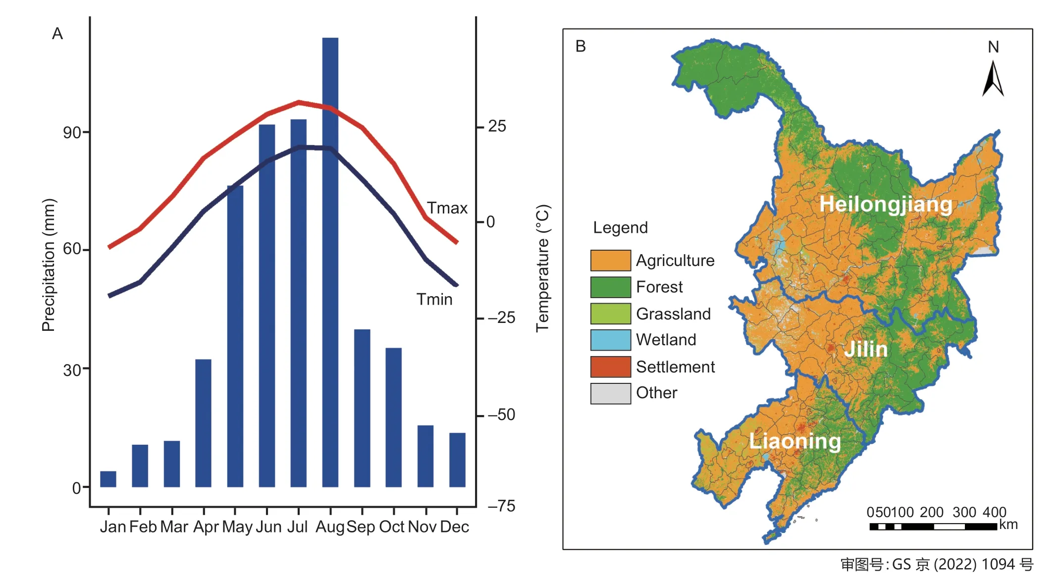
Fig.1 Monthly precipitation,average daily maximum (Tmax) and minimum temperature (Tmin) (A) and land cover (B) in Northeast China in 2015.

2.2.NUE data and covariates

Two indicators of NUE long-term trends were used: PFPNand PNBN(Dobermann 2007).

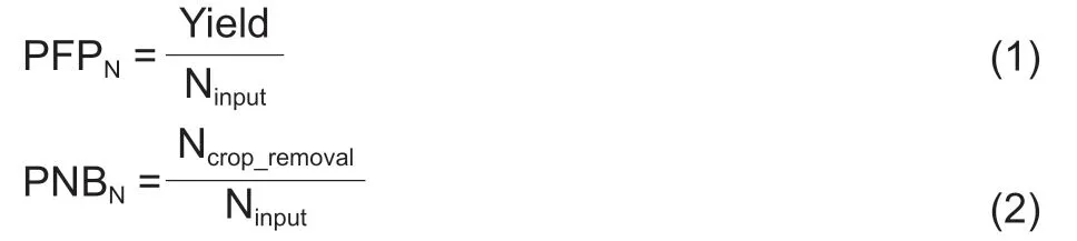
where Yield refers to the economic yield of crop with applied;Ninputis the total amount of nitrogen applied to the field from different sources (chemical fertilizer,manure,cake fertilizer and straw) and Ncrop_removalis the total removal in aboveground crop biomass with nitrogen applied.

The total number of observations for each indicator was 4 687 (i.e.,the product of years and counties).Economic yield and planting area were obtained for 10 crops: cereals,beans,tubers,oil crop,sugar crop,fiber(including cotton),tobacco,vegetables,melons and fruits. Crop yields of the main harvested products were measured as fresh weight for vegetables,melons and fruits,dry matter for others. Chemical N fertilizer sources were single N fertilizer and compound N fertilizer. Manure fertilizers came from cattle,pigs,sheep,poultry,horse,donkey,mule and humans. More details about computing NUE indicators are given in Heet al.(2018). The county data for NUE calculation were obtained from the Municipal Statistical Yearbook (1991-2016) of Northeast China.

Explanatory variables (i.e.,covariates) contained topography (6 covariates),crop covariates (enhanced vegetation index (EVI,6 covariates),crop types (10 covariates,as listed above),soil types (17 covariates,which were aggregated from 118 soil sub-types based on reference groups of the World Reference Base),soil properties (34 covariates),climate (12 covariates),economy (1 covariates) and AMP (2 covariates). These were obtained from the Climatic Research Unit (2015),Harriset al.(2014),the National Bureau of Statistics of China (1991-2016) and published articles (Shangguanet al.2014;Henglet al.2017;de Sousaet al.2020).More details about the explanatory variables including abbreviations can be found in Appendix B. All explanatory variables available in raster maps were aggregated to county scale by taking the spatial average over agricultural land (obtained by land cover maps during 1992-2015 from the European Space Agency Climate Change Initiative Land Cover (ESA 2021)). Most covariates were dynamic and varied between years,except for the enhanced vegetation index (for which we took long-term averages for each of the two-month time periods within a year,thus capturing seasonal variation),topography and soil covariates,which were considered static because these covariates had negligible temporal variation during the period studied. Crop and soil types were transformed to continuous-numerical variables by computing area proportions. Climatic variables (excluding night and daytime temperature,which were only available as annual values) were computed for the crop growing season (March-October) (Rayet al.2015). A total of 88 explanatory variables were employed to analyse and explain the spatial-temporal variation of PFPNand PNBN.

The pre-processing of the initial data set before computing NUE indicators and building models was as follows: (a) filling missing data and covariates in absent years,either by consulting statistical yearbook/published literature,supplementing missing values by mean values of adjacent years (if the time gap was relatively small),or by using data from neighbouring counties. For covariates,we used the ‘poly2nb’ function of the ‘spdep’ package(v.1.1-5) to fill gaps;(b) we flagged suspicious values(i.e.,outliers that are 10 times larger or smaller than that of adjacent years) and double-checked the reference data and compared them with other available data.

2.3.SMLR and RF models

The SMLR and RF models were used to help to summarize and understand spatial and temporal patterns of NUE. Although they cannot detect causal influences(only correlations instead),they provide insight into the causes of the variation by quantifying the importance of explanatory variables.

SMLR modelMultiple linear regression models simulate the linear relation between a dependent variable (i.e.,NUE indicator) and explantory variables. Stepwise regression was used to select explanatory variables automatically and simplify the initial model that used all covariates. We used the Bayesian information criterion(BIC) and both direction for variables selection,as implemented in the ‘stepAIC’ function in the ‘MASS’package,v.7.3-53 of the R language for statistical computing (R Core Team 2021). A common problem of SMLR is multicollinearity (highly linearly correlated explanatory variables),which can be detected using the variance inflation factor (VIF). A rule of thumb is that the VIFs of all covariates used in the model should be smaller than 10 to avoid multicollinearity (Kutneret al.2004). If the highest VIF was greater than 10,we deleted the corresponding explanatory variable and refitted the model.This procedure was repeated until all VIFs were below 10.Next,we used the ‘confint’ function in the ‘stats’ package(v.3.6.2) to obtain confidence intervals of the remaining explanatory variables coefficients. Insignificant variables(i.e.,P＞0.05) were deleted from the model,again in a stepwise manner. More details about the model building process are given in Appendix C.

Bivariate correlations between covariates and dependent variables were also computed and examined since this was helpful to understand the correlation of the data and interpret results. Corresponding scatter plots were plotted in a single figure using the ‘chart.Correlation’function of the ‘PerformanceAnalytics’ package,v.2.0.4.Multiple linear regression assumes that the regression residuals are independent and identically distributed Gaussian variables. The normality assumption was evaluated by computing the studentized residual,the histogram of which is generated in the ‘residplot’ function(Kabacoff 2011),which superimposes a normal curve,kernel density curve and rug plot,visually reflecting how close model errors are to a normal distribution. To make the regression coefficients of the final model more interpretable,all explanatory variables were standardized to zero mean and unit standard deviation prior to model calibration,using the ‘scale’ function in the base package of R. As a result,the regression coefficients describe the expected change in the dependent variable for a standard deviation change in an explanatory variable,holding the other explanatory variables constant. This is the simplest method to obtain the relative importance of explanatory variables. In this study,we used the method of relative weights (abbreviated as ‘relweights’) to obtain the relative importance of explanatory variables (‘relweights’ function,Kabacoff 2011). This method closely approximates the average increase in the model efficiency coefficient(MEC) (see eq.(4) in Section 2.4) obtained by adding an explanatory variable across all possible sub-models.Another method (Lindeman,Merenda and Gold (LMG))is averaging over orderings proposed by Lindemanet al.(1980),which was calculated using the ‘calc.relimp’function of R package ‘relaimpo’ v.2.2-3 (Grömping 2006).

RF modelThe RF algorithm,developed by Breiman(2001),tends to have higher accuracy compared with other approaches (Henglet al.2015). It belongs to the family of ensemble machine learning algorithms that predicts a dependent variable (in this case a NUE indicator) from a set of explanatory variables (training data) selected randomly using a bootstrapping technique(sampling with replacement). In this way,it generates multiple trees in the training procedure without pruning(reducing the number of trees) and aggregates the results.Each tree in the forest is less correlated with other trees because only random subsets of covariates are included in each tree,which increases accuracy (Gislasonet al.2006). For each tree,there are two datasets: the “in-bag”data for model training that contained two thirds of the features data set and the “out-of-bag (OOB)” data to verify model error that contained the remaining one third of the features data (Fraiwanet al.2012). Three user-defined parameters are required in the RF model: the number of trees (ntree,500,following a rule-of-thumb),the number of variables as explanatory variables to grow in each tree(mtry,32,1/3 of explanatory variables),and the minimum size of terminal nodes (node size,5) (Liuet al.2015).Default values of these parameters were used in this study. Themtryparameter determines the strength of each tree and the correlation among trees in the model,meaning that the strengths of the individual trees and the correlations among all trees increase asmtryincreases(Prasadet al.2006;Peterset al.2008).

The complexity of the RF model means that it has a ‘black box’ character,although variable importance ranking is possible with RF and provides valuable information about what drives the model (Breiman 2001).Two variable importance methods in the ‘randomForest’package v.4.6-14 are the mean increase in mean square error (unscaled %IncMSE) and total decrease in node impurities (IncNodePurity). For convenience of presentation,we normalized the variable importance of the most important explanatory variables of the RF models (using an equal number of variables as used in the corresponding SMLR model) to sum to 100%.Computations of the RF model can be costly but this has been greatly improved with the development of the‘RANdom forest GEneRator’ (‘ranger’ v.0.12.1) package,which has good scaling properties with the number of features,samples,trees,and features tried for splitting(Wright and Ziegler 2017). The ‘ranger’ package uses unscaled permutation and node impurity methods for ranking variable importance (Nicodemuset al.2010).

2.4.Validation/Accuracy assessment

Cross-validation is a popular approach for assessing and selecting predictive models. In this study,we used 10-fold cross-validation by the ‘shrinkage’ function (Kabacoff 2011) for SMLR models and the ‘RFcv’ function in the‘spm’ package v.1.2.0 for RF models. In 10-fold crossvalidation,the sample is divided into 10 subsamples.Each of the 10 subsamples serves as a hold-out group and the combined observations from the remaining 9 subsamples serves as the training group. The performance for the 10 prediction equations applied to the 10 hold-out samples are recorded and then averaged(Kabacoff 2011). The model validation metrics were the mean error (ME),root mean squared error (RMSE),normalized RMSE (nRMSE),model efficiency coefficient(MEC) and Lin’s concordance correlation coefficient(LCCC) (Lin 1989). These are computed as follows:

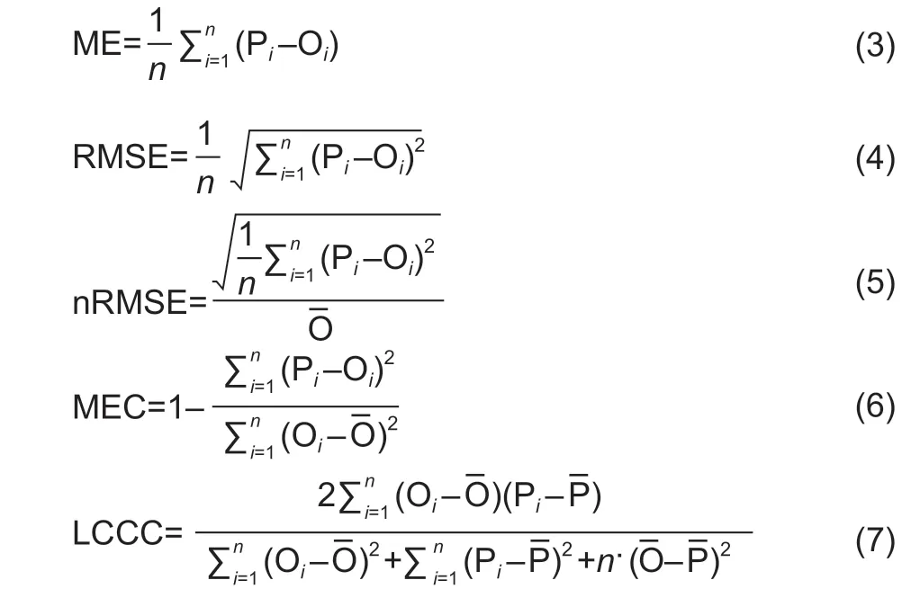
wherenis the number of observations;PiandOiare the predicted and observed NUE values for observationi,respectively,and -Pand -Oare the means of the predicted and observed NUE values.

We consider nRMSE≤15% as good agreement;15-30% as moderate agreement;and ≥30% as poor agreement (Liuet al.2013). If MEC is over 0.90,this indicates good agreement between observations and predictions (Aghdaeiet al.2017). According to Ichamiet al.(2019),a model with a MEC higher than 0.3 could still be a useful model in this domain of science.An LCCC smaller than 0.90 is considered as poor agreement,0.90-0.95 as moderate agreement,0.95-0.99 as substantial agreement,and larger than 0.99 as almost perfect agreement (de Beaufortet al.2017).

3.Results

3.1.Spatial and temporal variations of NUE indicators from 1990 to 2015

Spatial and temporal variations of PFPNIn order to depict spatial patterns of county-level PFPNin Northeast China from 1990 to 2015,the PFPNwere grouped into five categories: very low (＜25 kg kg-1yr-1),low (25-35 kg kg-1yr-1),moderate (35-45 kg kg-1yr-1),high (45-60 kg kg-1yr-1),and very high (＞60 kg kg-1yr-1) (Fig.2).Overall,most counties in Heilongjiang Province had higher PFPNand in Jilin Province had lower PFPNvalues.Over the first four periods,more counties had very low PFPN(increasing from 32 to 43 counties) and moderate PFPNvalues (increasing from 37 to 52 counties),and fewer counties had high PFPN(decreasing from 34 to 26 counties) and very high PFPNvalues (decreasing from 32 to 14 counties). In the fifth period,fewer counties (23 counties;within Jilin Province,southeast and northwest of Liaoning Province) had PFPNvalues at a very low level,and more counties (41 counties;within Heilongjiang Province,middle and southwest of Liaoning Province) had PFPNvalues at a high level.

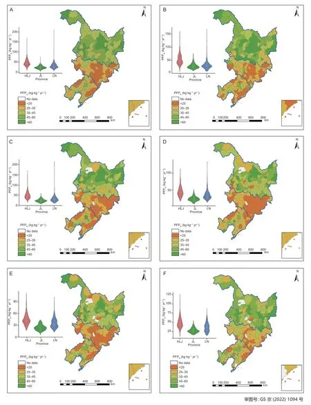
Fig.2 Spatial distribution of county-average PFPN in Northeast China for six time periods in 1990-2015 (A),1990-1995 (B),1996-2000 (C),2001-2005 (D),2006-2010 (E) and 2011-2015 (F). HLJ,Heilongjiang;JL,Jilin;LN,Liaoning.

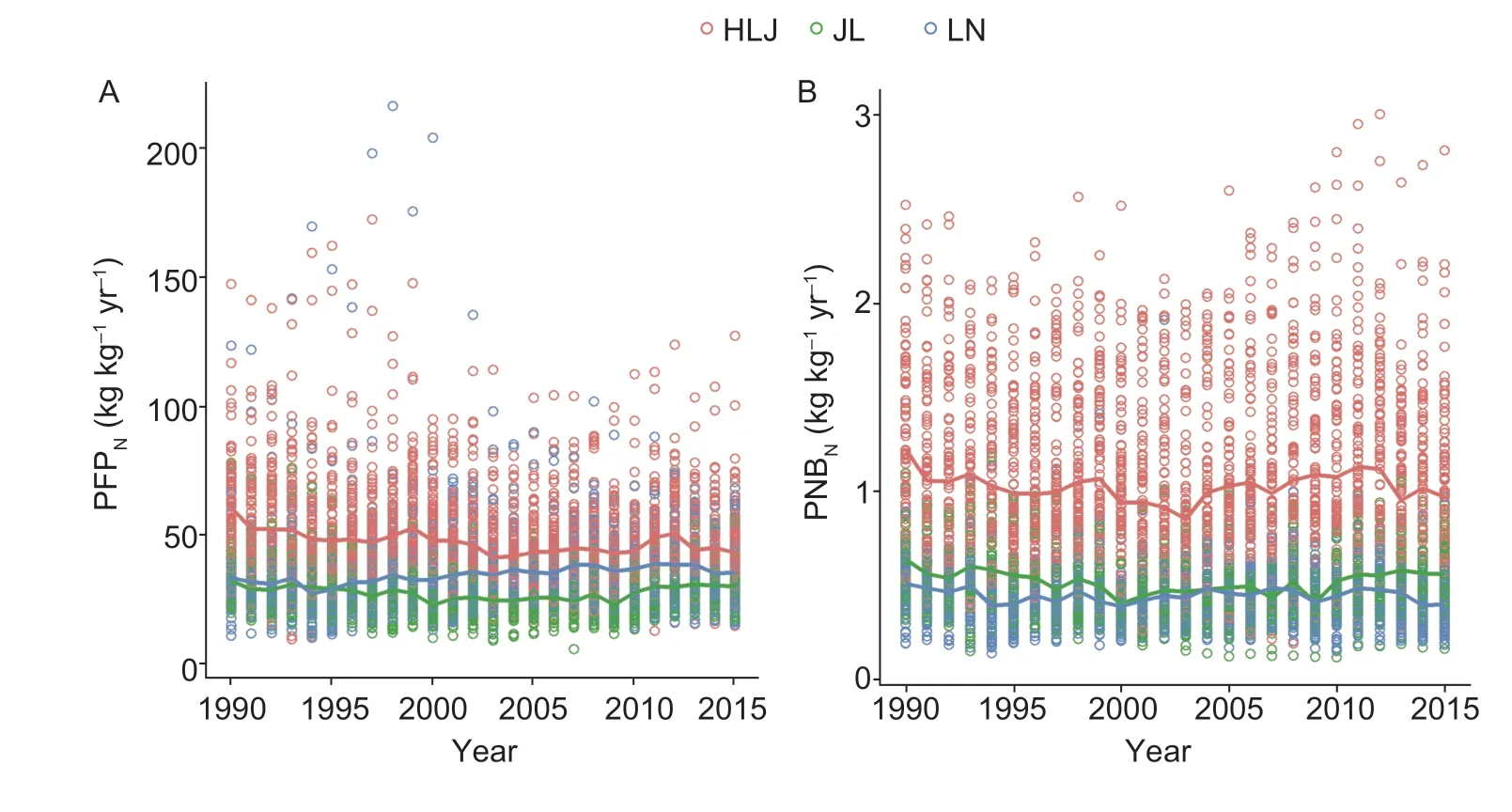
Fig.3 Temporal variation of partial factor productivity of nitrogen (PFPN;A) and partial nutrient balance of nitrogen (PNBN;B) in Northeast China from 1990 to 2015. The solid red,green and blue lines represent the aggregated provincial nitrogen use efficiency indicators of Heilongjiang (HLJ),Jilin (JL) and Liaoning (LN) provinces,respectively,which was computed by averaging over counties (Sum of yields/N of crops removal in each county divided by the sum of N input).

The temporal variation of PFPNvaried between counties in Northeast China (Figs.3-A and 4-A). On a county scale,we selected the five biggest-area counties in each province for display in Fig.4. Their temporal variation trends from 1990 to 2015 fluctuated more than the provincial trend. Overall,they can be divided into two types (Fig.4-A): (1) decrease in most counties (the average annual growth rate ranged from -6.1 to -0.1%);(2) increase in Huma County of Heilongjiang Province,Beipiao County of Liaoning Province and Antu County of Jilin Province (the average annual growth rate ranged from 0.2 to 2.3%).

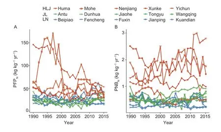
Fig.4 Temporal variation of partial factor productivity of nitrogen (PFPN;A) and partial nutrient balance of nitrogen (PNBN;B) in fifteen counties in Northeast China from 1990 to 2015. The red,green and blue colour represents the province of Heilongjiang (HLJ),Jilin (JL) and Liaoning (LN),respectively. The counties in the scatter plot were the five biggest-area counties of each province.

Spatial and temporal variations of PNBNOverall,the PNBNincreased from south to north in the study area in the period 1990-2015 (Fig.5-A). This might be related to the spatial patterns of crop removal N and N input: these were lower in the north of Northeast China (Appendix D).PNBNwas divided into five classes: very low (＜0.45 kg kg-1yr-1),low (0.45-0.65 kg kg-1yr-1),moderate (0.65-1.00 kg kg-1yr-1),high (1.00-1.50 kg kg-1yr-1),and very high(＞1.50 kg kg-1yr-1). More counties had very low and low PNBN,and fewer counties had high and very high PNBNfrom 1990 to 2005. In contrast,from 2006 to 2015,fewer counties had PNBNat a very low level,and more counties had PNBNat moderate and high levels.

The trend of PNBNvariation from 1990 to 2015 was different among the counties (the five biggest-area counties from each province were selected and plotted in Fig.4-B): PNBNdecreased in most counties (the average annual growth rate ranged from -3.8 to -0.3%);it had no notable change in Beipiao County of Liaoning Province and Mohe County of Heilongjiang Province (～0.0% of the average annual growth rate);and increased in Fengcheng County of Liaoning Province,Wangqing and Antu counties of Jilin Province,and Huma County of Heilongjiang Province (the average annual growth rate ranged from 0.3 to 3.0%).

3.2.Prediction models and performance evaluation

SMLR modelSummary statistics of the NUE indicators and explanatory variables included in the final SMLR model are listed in Table 1. The PFPNand PNBNvalues exhibited a slightly skewed distribution,with skewness and kurtosis coefficients of 2.01 and 11.52 for PFPN,and 1.38 and 4.65 for PNBN,respectively;and mean values of 40 and 0.75 kg kg-1yr-1(ranging from 5 to 216 kg kg-1yr-1for PFPN,and from 0.12 to 3.00 kg kg-1yr-1for PNBN),respectively,which were higher than their standard deviations (19 and 0.46 kg kg-1yr-1,respectively).

The regression coefficients and VIF of the SMLR models are shown in Table 2. We standardized the explanatory variables to compare regression coefficients.All explanatory variables in the final model affected the NUE indicators significantly (P＜0.01) and had a VIF less than 10;among them,seven explanatory variables had a negative impact and ten showed a positive influence on PFPN;for PNBN,there were seven explanatory variables with a negative and eight with a positive influence.The studentized residuals were not strictly Gaussian distributed,which suggests that the normality assumption was not perfectly satisfied (Fig.6).

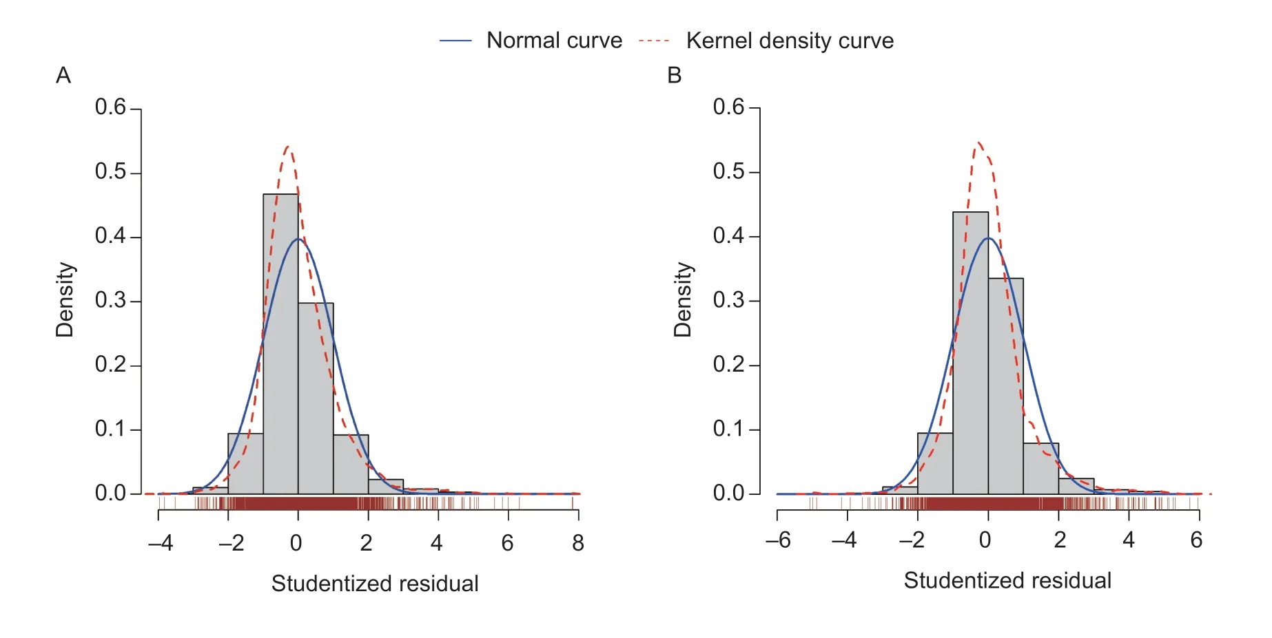
Fig.6 Distribution of residual standard errors for partial factor productivity of nitrogen (PFPN) model (A) and partial nutrient balance of nitrogen (PNBN) model (B).

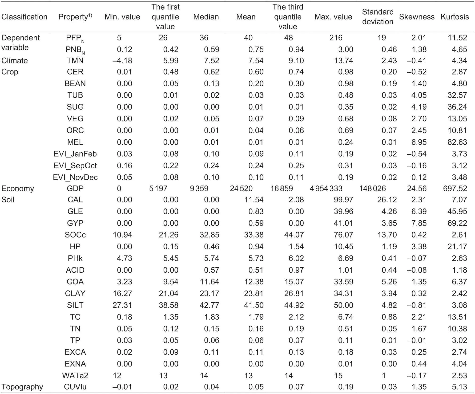
Table 1 Descriptive statistics of nitrogen use efficiency indicators and explanatory variables in the stepwise multiple linear regression model

RF modelIt took a while for the RF model to stabilize(Appendix E). The MSE,RMSE and MEC converged to 57 (kg kg-1yr-1)2,7.5 kg kg-1yr-1,0.84 for PFPN,and 0.02 (kg kg-1yr-1)2,0.15 kg kg-1yr-1,0.89 for PNBN,respectively,using 500 trees. This showed that a forest with 500 trees was large enough to get stable results.In this study,we therefore followed the rule-of-thumb that there should be at least 500 trees in a forest,even though a forest with 50 trees provided good results(Appendix E).

Accuracy comparison between SMLR and RF modelsRF used all 88 variables in a ‘black box’approach while the SMLR models used fewer covariates.Thus,the latter were easier to interpret. The model performance metrics for each model were similar between 10-fold cross-validation and the internal model (original model built using the complete dataset)(Table 3),indicating there was no over-fitting problem.SMLR and RF models explained 44 and 84% of the PFPNvariance,and 67 and 89% of the PNBNvariance,respectively. Therefore,the RF model had much higher accuracy. The ME was close to zero and revealed unbiased predictions for all models. Regarding other model performance metrics,the RF models showed moderate performance,while SMLR models had poor performance,especially for PFPN. The scatter and density plots of observations and predictions also showed that the RF models had smaller prediction errors than SMLR models (Fig.7-F and H). As with most statistical prediction methods,both models smooth the reality and underpredict high extremes and overpredict low extremes.

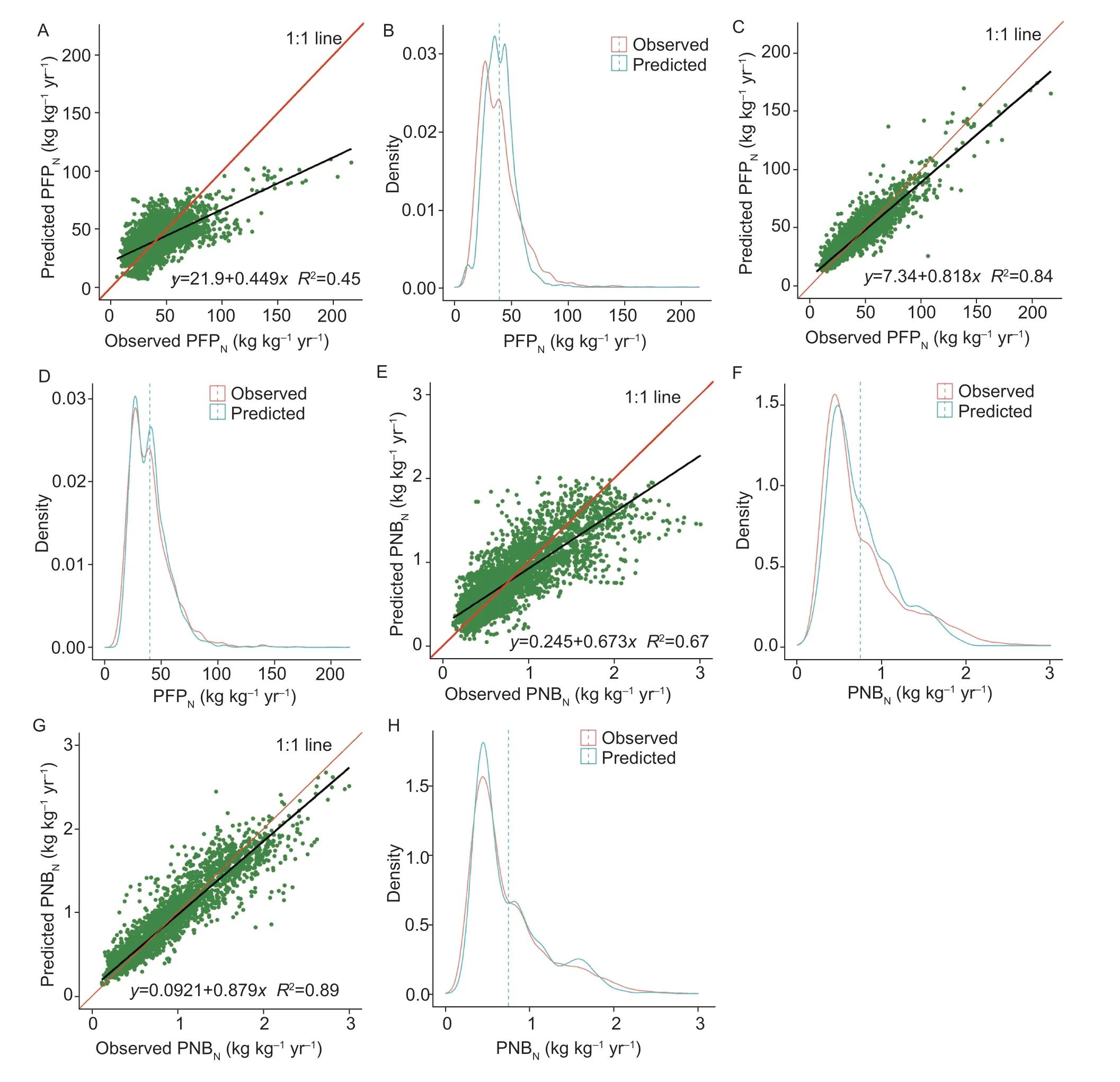
Fig.7 Scatter plots and Kernel density plots of observed and predicted partial factor productivity of nitrogen (PFPN) (A,B for SMLR model and C,D for RF model) and partial nutrient balance of nitrogen (PNBN) (E,F for SMLR model and G,H for RF model). The dotted line shows the average value in Kernel density plots;the average values of observed and predicted variables were the same.

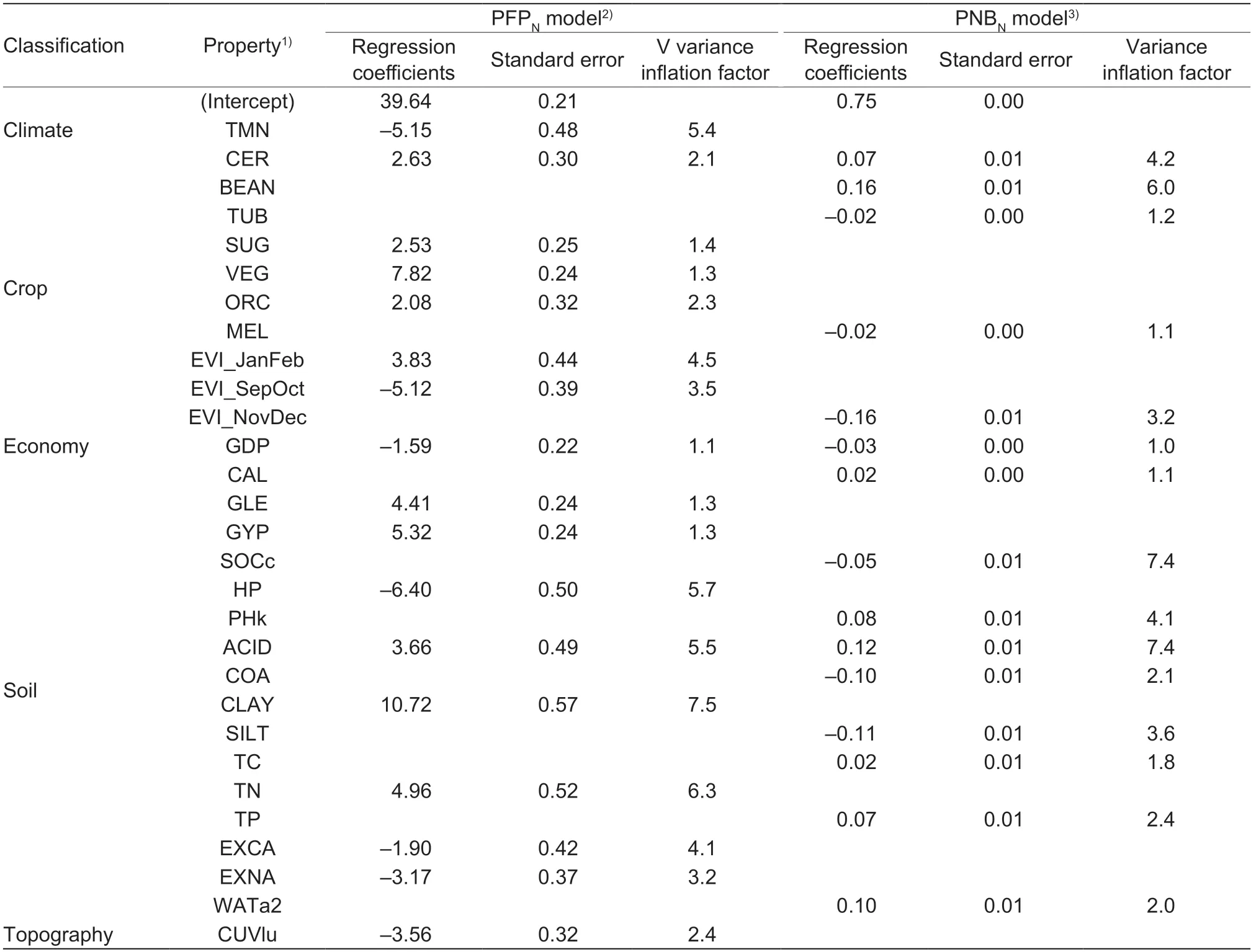
Table 2 Regression coefficients and variance inflation factor of the stepwise multiple linear regression models

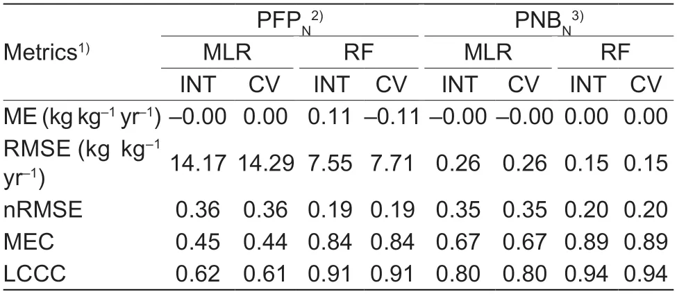
Table 3 Model performance and cross-validation metrics of stepwise multiple linear regression and Random Forest models

3.3.Relative importance of explanatory variables

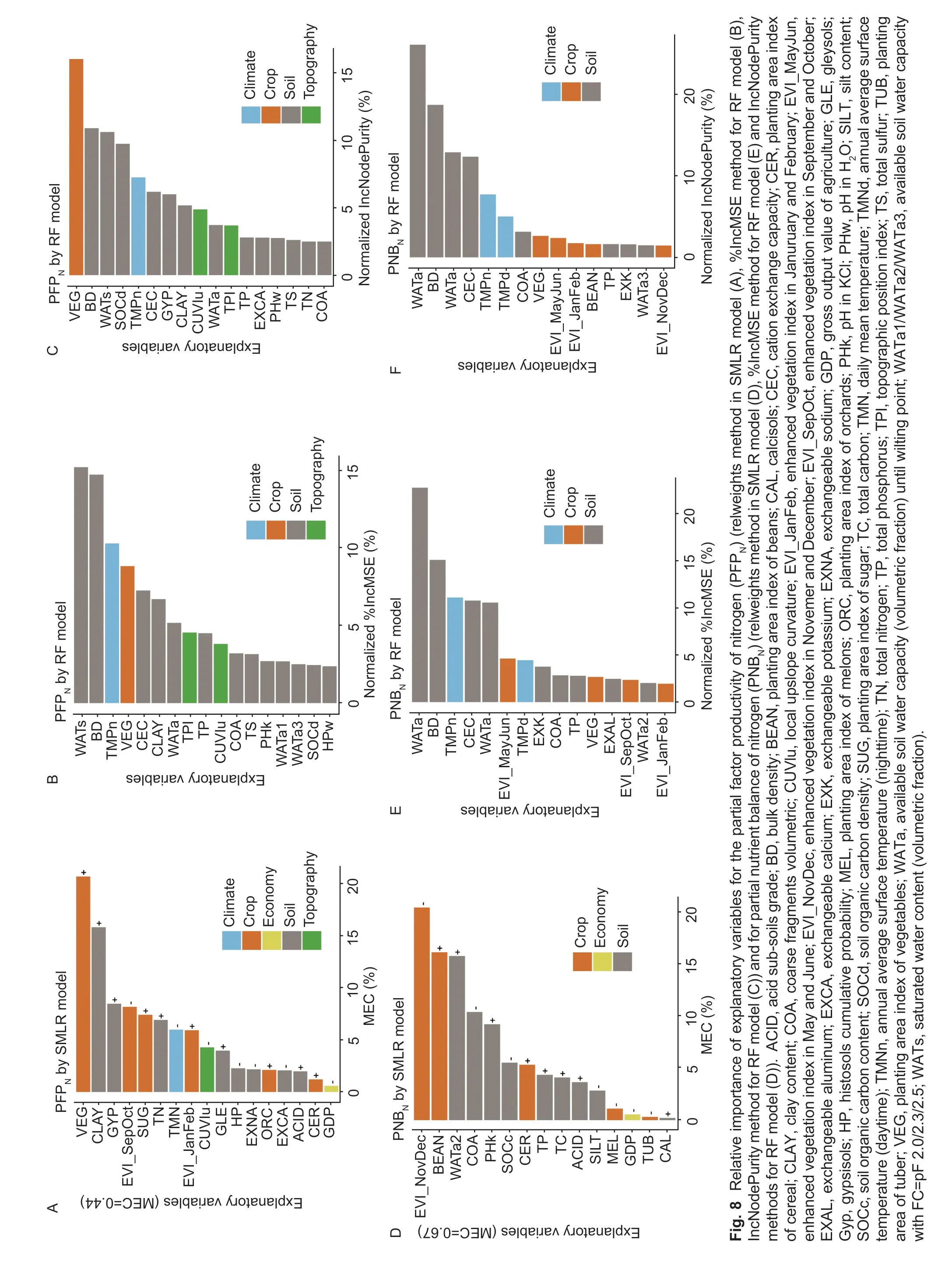
Here,we only show the variable importance results for the relweights method in the SMLR model,and the%IncMSE and IncNodePurity methods in the RF model(Fig.8). Results of the other variable importance methods(LMG and ranger) were similar to the above methods,so they are provided only in Appendix F.

Relative importance of explanatory variables for PFPNFor PFPN,the results of the relweights method suggested that crop and soil covariates had similar importance in the SMLR model accounting for 46 and 44% of the MEC,respectively (Fig.8-A). The main crop covariates were planting area index of vegetables(21%),sugar (7%),EVI in September &October (8%),EVI in January &February (6%). Most of the covariates had a positive influence on PFPN(EVI in September &October was an exception). Major soil covariates with positive regression coefficients were clay content (16%),gypsisols (8%) and total (7%). Soil covariates had more positive explanatory variables than negative variables(i.e.,histosols cumulative,exchangeable sodium and exchangeable calcium). Climatic (i.e.,annual average daily minimum temperature 6%),topographic (i.e.,local upslope curvature 4%) and economic variables (i.e.,agricultural GDP 0.6%) had negative impacts on PFPN.

The %IncMSE and IncNodePurity methods showed similar results for variable relative importance (Fig.8-B and C). Soil covariates accounted for the highest importance (73% for the normalized %IncMSE and 68%for the normalized IncNodePurity methods;e.g.,bulk density 15 and 11%,saturated water content 15 and 11%,soil organic carbon density 2 and 10%,CEC 7 and 6%,clay content 7 and 5% for %IncMSE and IncNodePurity,respectively). Crop covariates (planting area index of vegetables) were less important than soil covariates,accounting for 9 and 16% for the %IncMSE and IncNodePurity methods,respectively. Topography ranked the third (i.e.,local upslope curvature 5%,topographic position index (TPI) 4% for %IncMSE,and the same for IncNodePurity) and climate factors the fourth (i.e.,annual average night land surface temperature 10 and 7% for%IncMSE and IncNodePurity,respectively).

There was a large difference in the variable importance between the SMLR and RF models. The relative importance of soil covariates in the RF model was much higher than in the SMLR model,while that of crop covariates was much lower. For individual variables,planting area index of vegetables and soil clay content had higher relative importance in the SMLR than in the RF model. In contrast,the relative importance of other soil covariates (e.g.,bulk density,saturated water content,soil organic carbon density and CEC) and minimum temperature was higher in the RF than in the SMLR model.

Relative importance of explanatory variables for PNBNFor PNBN,the relweights method showed that soil covariates had the highest importance in the SMLR model (accounting for 56% of the MEC,e.g.,available soil water capacity (with FC=pF 2.3) 16%,coarse fragments(＞2 mm) 10%,pH (in KCl) 9% and soil organic carbon content 6%),followed by crop covariates (43%,e.g.,EVI in November &December 20%,planting area index of beans 16%,cereal 5%) (Fig.8-D). Economic covariates had the least influence,accounting for 0.5% (i.e.,agricultural GDP) of the MEC. Most soil covariates had a positive influence on PNBNin the SMLR model,however coarse fragments,soil organic carbon content and silt content had negative effects (Fig.8-D). EVI in November&December and planting area index of melons and tubers also decreased PNBN,while planting area index of beans and cereals led to an increase. Agricultural GDP had,unexpectedly,a slight negative impact on PNBN.

The variable relative importance of the %IncMSE and IncNodePurity methods for PNBNwere similar(Fig.8-E and F). Soil covariates accounted for the highest importance (71% of the normalized %IncMSE and 77% of the normalized IncNodePurity methods;e.g.,saturated water content 23 and 27%,bulk density 14 and 15%,available soil water capacity until wilting point 11 and 14% and CEC 11 and 13% for the %IncMSE and IncNodePurity methods,respectively),followed by climate factors (17 and 14% for the %IncMSE and IncNodePurity methods,respectively,i.e.,annual average night land surface temperature 12 and 8% and annual average surface temperature at daytime 5 and 6% for the %IncMSE and IncNodePurity methods,respectively)and crop covariates (12 and 10% for %IncMSE and IncNodePurity,respectively,e.g.,EVI in May &June 4 and 2% for the %IncMSE and IncNodePurity methods,respectively) (Fig.8-F).

The main difference in the variable relative importance between the SMLR and RF models for PNBNwas that the RF model had higher relative importance of soil and climatic covariates,and lower relative importance of crop covariates. For individual variables,the relative importance of EVI in November &December and planting area index of beans were higher in the SMLR than in the RF model,while the relative importance of saturated water content,bulk density,CEC and annual average surface temperature was higher in the RF than in the SMLR model.

4.Discussion

4.1.Spatial and temporal variation of NUE indicators

Most counties in Jilin and Liaoning provinces had higher crop yields than most counties in Heilongjiang Province where N application was lower (Appendix D). Some counties such as Yichun and Qiqihaer in Heilongjiang Province performed well since they produced higher yields with lower N inputs. These counties may have had high soil fertility,and good water and nutrient management.Management practices in these counties could be shared to support farmers in other counties,although it should be noted that soil depletion may still occur in the long run. During the 1990-2010 period there was an overall reduction in PFPN: more counties had very low and moderate PFPNlevels,while less counties had high and very high PFPNlevels. After that period,the situation improved: less counties had PFPNat very low levels (e.g.,northeast of Jilin Province),and more counties had PFPNat a high level (e.g.,middle and southwest of Liaoning Province). Zhuet al.(2018) also found that PFPNdecreased from the 1980s to the 2000s. Therefore,with the NUE increasing in Jilin and Liaoning provinces,the spatial patterns of PFPNmight change in the future.

Heet al.(2018) reported that PNBNin Northeast China was 0.50,0.45 and 0.50 kg kg-1yr-1in the 1990s,2000s and 2010s,respectively. The present study revealed a similar trend,but the values were higher,i.e.,0.76,0.72 and 0.78 kg kg-1yr-1,respectively. The differences are likely caused by the fact that Heet al.(2018) considered additional N input sources (symbiotic and non-symbiotic fixation,dry and wet atmospheric deposition,irrigation water and crop seed). Fixenet al.(2015) suggested that a PNBNof 0.7-0.9 kg kg-1is a typical level (with chemical and organic fertilizers as N inputs). In our study,while it is a good sign that more counties reached a moderate PNBNlevel during the final time period,other counties still had lower levels. These counties require assistance as advanced management could improve efficiency or increase soil fertility. EU Nitrogen Expert Panel (2015)observed that a PNBNof 0.7-0.9 kg kg-1indicates a balanced N fertilization,and suggested target values between 0.5-0.9 kg kg-1. In our study,64 counties were in this target interval in 2015. The EU target is based on total N inputs,while we only included chemical and organic fertilizers. The average PNBNin Heilongjiang Province was higher than 1,indicating that the soil is in a mining situation.Meanwhile,this specific situation is unsustainable. PNBNwas lower than 0.55 kg kg-1in Jilin and Liaoning provinces,suggesting avoidable N losses were occurring and the NUE should be improved (Snyder and Bruulsema 2007).

4.2.Performance comparison between SMLR and RF models

In the SMLR models,regression coefficients are dependent on the unit of each explanatory variable. The SMLR models used 17 and 15 explanatory variables for PFPN/PNBN,but the RF model used all the variables in a ‘black box’ (no closed-form expression for the prediction equation). In this perspective,the SMLR model was simpler than the RF model and easier to explain.However,the RF model has a higher accuracy and ability to model complex interactions between variables(Grömping 2009;Richardsonet al.2017). Limitations of the SMLR and RF models are that these models are usually only effective within the range of covariate values exhibited by the training data,that relations found are empirical rather than causal and that overfitting may occur in instances where noisy data are being modelled (Henglet al.2015). Therefor it should be kept in mind that our prediction model should not be applied out of range. For model performance metrics (except ME),RF models were more predictive than SMLR models,especially for PFPN. This suggests that non-linear relationship between dependent and explanatory variables was more important for PFPNthan for PNBN. The statistical model for predicting NUE at farm level had an MEC of 0.77 (Ramírez and Reheul 2009). Liuet al.(2020) obtained an NUE model at provincial scale with an MEC of 0.74. They were less predictable than the RF model in this article (MEC of 0.84/0.89). In principle,our RF model is especially good at predicting NUE at county level in Northeast China which is consistent with training data. Predictions outside the area of applicability should be handled with care or be left out from further consideration because the environmental properties differ too strongly from those observed in the training data (Meyer and Pebesma 2021).

4.3.Relative importance comparison of explanatory variables

Relative importance of variables for PFPNFor PFPN,the crop covariates (e.g.,planting area index of vegetables) were the most important factors for the relweights and %IncMSE methods,while they ranked the second in the IncNodePurity method. In particular,planting area index of vegetables had a highly positive influence on PFPNin the SMLR model. The yield per unit of vegetables (measured as fresh weight) was higher than that of other crops (measured as dry matter). This is not surprising given that fresh weight is typically larger than dry matter weight. However,this does not mean that more vegetables should be grown,because this would neither increase the nutritious value nor promote food security. Besides that,the EVI was an important factor in the relweights method. Although they are all negatively correlated with PFPN,but the equation coefficients showed that EVI in September and October had a negative influence while EVI in January and February had a positive influence on PFPNin the SMLR model.

Soil covariates were the most important variables for the IncNodePurity method,while they were the second most important for the relweights and %IncMSE methods.The representative covariates in the SMLR model were clay content,gypsisols and total N. Hamoudet al.(2019)indicated that an increase in soil clay content improved rice root morphology and NUE. In addition,more clay means less leaching because leaching mainly takes place in sandy soils. Cambisols,soil organic carbon density and the amount of phosphorus (Olsen method) were the representative variables in the %IncMSE method of the RF model. The IncNodePurity method suggested that bulk density,saturated water content,soil organic carbon density and CEC were the main soil covariates.These covariates are important soil properties,which have a direct influence on N uptake by crops and soil N mineralization (Ishaqet al.2002). Saturated water content reflects the pore status of the soil and the maximum water holding capacity,which is beneficial to NUE (Iqbalet al.2019). The high saturated water content (43-56%) also reflects high soil organic matter.CEC gives insight into the fertility and nutrient retention capacity of the soil,because exchangeable cations are the most important source of immediately available K,Ca and Mg (Mukhopadhyayet al.2019). Soil covariates had more positive explanatory variables than negative variables (i.e.,histosols cumulative,exchangeable sodium and exchangeable calcium). Liuet al.(2020)also indicated that histosols cumulative had a negative influence on yield,because histosols typically are poorly drained soils,where organic matter accumulation is greater than mineralization.

The relative importance of climate factors was similar in the relweights and IncNodePurity methods. In the relweights method of the SMLR model,annual average daily minimum temperature had negative impacts on PFPN,and in the RF model,annual average surface temperature at night was also important. Temperature is among the key driving factors of crop yield variability(Zscheischleet al.2017). The temperature in Northeast China is lower than in other regions of China and the minimum night land surface temperature restricts the PFPNby limiting crop growth and N absorption (Jinet al.2017). Chenet al.(2011) found that daily minimum temperature was the dominant factor in corn production,especially in May and September.

The economic variable (i.e.,agricultural GDP) was more important in the IncMSE method of the RF model than in the relweights method of the SMLR model. Agricultural GDP refers to the total amount of all agricultural products expressed in monetary currency,reflecting the general trend of agricultural production in a certain period,which is related to crop types,crop yield and market price. This influences NUE at a macroeconomic level. In this study,agricultural GDP per unit of planting area,rather than per capita,was used to better reveal the agricultural productivity and explore the relationship with NUE. Higher agricultural GDP promotes the improvement of mechanization,and this pays off in a higher yield and NUE. Conversely,once the agricultural GDP reaches a certain level,excessive fertilization might also cause reduced NUE. The non-linear relationship between agricultural GDP and PFPNexplained why agricultural GDP had a low importance in the SMLR model.

Topography was more important in the RF model than the SMLR model. Local upslope curvature and TPI were the main topographic covariates. Local upslope curvature is detrimental to PFPN. TPI measures the relative topographic position of a point as the difference between the elevation at this point and the mean elevation within a predetermined neighborhood (De Reuet al.2013). TPI could influence climate variability (temperature,precipitation;Tanget al.2017) and N loss (Singhet al.2019).

The relative importance of soil covariates in the RF model was much higher than in the SMLR model while that of crop covariates was much lower. This may be because crop covariates tend to be more linearly correlated with PFPN,while soil covariates are more complex and tend to be nonlinearly correlated. For individual variables,planting area index of vegetables had higher relative importance in the SMLR than in the RF model,because vegetables had higher PFPNthan other crops (＞ 80 kg kg-1in Liet al.2017). The soil clay content is also more important in the SMLR model. This might be because the range of soil clay content (16-34%) in this study had a linear relation with PFPN,so its influence is well-represented in the SMLR model. The relative importance of minimum temperature was higher in the RF than in the SMLR model. This might be because the relationship between temperature and NUE is nonlinear. Penget al.(2004) showed that increased night temperature decreased rice yields,which was associated with global warming. In contrast,Jinet al.(2017) indicated that higher NUE and rice yield could be obtained with a combination of higher effective temperature and fewer sunshine hours during the entire growth period in Northeast China.

Relative importance of variables for PNBNFor PNBN,three methods showed that soil covariates were the most important variables (＞50%). In the relweights method,available soil water capacity and pH had a positive influence while coarse fragments and soil organic carbon content had a negative impact on PNBN. Panet al.(2020)showed that greater water holding capacity improved maize growth and thus enhanced N absorption and accumulation by plants. Table 1 shows that the minimum pH was 4.73,so soil acidification of croplands decreased NUE (Panet al.2020),which can be overcome by the use of a combination of chemical and organic fertilizers(Miaoet al.2011). Coarse fragments increase the risk of N loss and ammonia volatilization,and thus reduce crop NUE (Penget al.2015). The saturated water content was very important in the %IncMSE and NodePurity methods.Saturated water content refers to the water content when all pores in the soil are filled with water. It is one of the soil moisture constants,reflecting the pore status of the soil and the maximum water holding capacity. Improved soil porosity is beneficial to NUE (Iqbalet al.2019). The bulk density,available soil water capacity until wilting point and CEC were also very important factors. CEC is a sign of soil fertility and nutrient retention capacity (Mukhopadhyayet al.2019). Soil water affects nutrient transformation from unavailable to available forms andvice versa,and thereby affecting the total nutrient uptake amount. It also influences the availability of applied nutrients and efficiency through its effect on various nutrient loss mechanisms such as volatilization,nitrification,and/or urease hydrolysis(Ullahet al.2019).

Crop covariates were second in importance in the three methods. EVI in November &December and planting area index of melons and tubers decreased PNBN,while planting area index of beans and cereal led to an increase. EVI in November &December also had a significantly negative correlation with PNBN(Appendix G).This is as expected because long winter dormancy inhibits crop growth and has a negative effect on PNBN(Gurunget al.2009). Melons have a lower N requirement per unit of economic yield than beans (Liuet al.2020),which explains their negative influence on PNBN. The planting area index of cereals was negatively correlated with PNBNbased on Pearson’s correlation,but showed positive influence in the SMLR model. This indicated that the influence of cereals on PNBNwas affected by other explanatory variables. Furthermore,cereal crops have various varieties. So NUE varied largely between different cereal crops and management practices (Xuet al.2014;Zhanget al.2015).

Climate factors were important in RF models according to the %IncMSE and NodePurity methods. Dinget al.(2018) also found that climate and soil variation were dominant factors driving N leaching. This is because temperature influences the N availability to crops and changes crop N removal and N losses from the plant-soil system (Lianget al.2018).

We had expected that increasing wealth would raise farmers’ investment in farming and the government’s attention to agriculture,and thus provide better agrotechnical services and increase NUE. Most countries,however,show an attenuated increase of maximum N removal from crops with increasing GDP,which adheres to the law of diminishing returns (Mogollónet al.2018).Despite that,the temptation of higher interests might lead to excessive fertilization and reduce NUE. In Japan,a negative relationship between GDP and maximum N removal from crops was found (Mogollónet al.2018).Proper guidance by the government and related scientific research workers is needed to avoid the negative effect of agricultural GDP.

The main difference in the relative importance of variables between the SMLR and RF models for PNBNwas that the RF model had higher relative importance of soil and climatic covariates,and lower relative importance of crop covariates. Similar to that observed for PFPN,this may be because crop covariates have a simple linear relationship with PNBNwhile soil and climate covariates are more complex and nonlinearly related with PNBN.For example,the relative importance of EVI in November&December and planting area index of beans were higher than 15% in the SMLR model,while they were lower than 5% in the RF model. In contrast,the relative importance of saturated water content,bulk density and CEC was higher in the RF than in the SMLR model;the annual average surface temperature was important in the RF model,but not in the SMLR model. This could be because EVI in November &December has a linear relation with PNBN,which SMLR captures well. However,soil covariates and temperature have a complex nonlinear relation with PNBN,by influencing N uptake and denitrification,which may explain why these were more important in the RF model (Fanet al.2014).

We compared different methods that quantify the relative importance of explanatory variables. Although the methods used for this are not entirely new,their comparison is rarely made and certainly not in the context of NUE modelling. Considering that the ‘ranger’ package is much faster,we found that the permutation and node impurity method used in the ‘ranger’ package were more efficient and trustworthy than in the ‘randomForest’package. However,it was difficult to recognize the negative or positive influence of covariates and interpret results with the ‘ranger’ package. More enhanced methods,such as deep learning,transfer learning,and wavelet phase harmonics (WPH) statistics are needed(Allyset al.2020). One thing that attracted our approval was that the %IncMSE method in the ‘randomForest’package and permutation method in the ‘ranger’ package were unscaled,because scaling of variable importance is misleading (Stroblet al.2009).

4.4.Crop-specific analyses at county scale

Many studies have focused only on a single crop or grain crop,and rarely included cash crops (Xuet al.2014;Liet al.2020). As a result,these studies do not reflect the entire local NUE trends,which inhibits their use for formulating appropriate policies and technical guidance.This study made up for these shortcomings by aggregating all crops and including crop types as explanatory variables.Analysis at a higher level of aggregation is important for decision and policy makers who often need integrated information that shows general patterns and trends (Liuet al.2020). However,in some cases decision makers may benefit from crop-specific analyses. Such analysis was beyond the scope of this work and is also hampered by the fact that crop-specific N application data at county scale are not readily available in the governmental database (i.e.,in the municipal and provincial Yearbook of Northeast China). Future research could look into ways to collect such data and apply a similar analysis as we did to reveal trends and patterns for specific crops and crop categories,such as staples and cash crops. Our analysis was also conducted at a county level,thus enabling recommendations and policies,such as N fertilization regulation,at a much finer scale than the provincial level.This is important because our results indicated that there were considerable differences in NUE trends between counties in the same province.

5.Conclusion

We performed a first and novel study analysing spatial and temporal variation of NUE at a county scale in three provinces in Northeast China using statistical regression.The NUE indicators decreased in most counties during the study period and were higher in Heilongjiang Province than in the other two provinces. The RF model was superior in performance than the SMLR model,indicating that many covariates had a non-linear relation with NUE. We note that both models smooth the reality and underpredict high extremes and overpredict low extremes. Considering that the ‘ranger’ package is much faster than the ‘randomForest’ package,we found that the permutation and node impurity methods in the ‘ranger’package were more efficient and trustworthy for analysing covariate importance in the RF model.

The relative importance of crop covariates was much higher in the SMLR than in the RF model,while soil and climatic covariates were more important in the RF model,indicating the difference between linear and nonlinear relationships between dependent and explanatory variables. These novel findings are particularly valuable when put into action in supporting land-use management and policymaking.

Acknowledgements

We thank Yi Qu (Research assistant,Institute of Agricultural Resources and Regional Planning,Chinese Academy of Agricultural Sciences) for collecting the county data. We are specially acknowledgeable financial support from the China Scholarship Council (CSC)(201903250115). This research was supported by the National Natural Science Foundation of China (31972515)and the China Agriculture Research System of MOF and MARA (CARS-09-P31).

Declaration of competing interest

The authors declare that they have no conflict of interest.

Appendicesassociated with this paper are available on http://www.ChinaAgriSci.com/V2/En/appendix.htm