Emergence of non-extensive seismic magnitude-frequency distribution from a Bayesian framework

Ewin Sánchez

Instituto de Investigación Multidisciplinario en Ciencia y Tecnología de la Universidad de La Serena 170000, Chile

ABSTRACT Non-extensive statistical mechanics has been used in recent years as a framework in order to build some seismic frequencymagnitude models.Following a Bayesian procedure through a process of marginalization,it is shown that some of these models can arise from the result shown here,which reinforces the relevance of the non-extensive distributions to explain the data(earthquake’s magnitude) observed during the seismic manifestation.In addition,it makes possible to extend the non-extensive family of distributions,which could explain cases that,eventually,could not be covered by the currently known distributions within this framework.The model obtained was applied to six data samples,corresponding to the frequency-magnitude distributions observed before and after the three strongest earthquakes registered in Chile during the late millennium.In all cases,fit parameters show a strong trend to a particular non-extensive model widely known in literature.

Keywords: Bayesian model;non-extensive statistics;frequency-magnitude distribution;earthquakes.

1.Introduction

Physics has long played an important role in understanding earthquake behaviour.There are aspects of materials physics such as elasticity theory,Rayleigh wave theory and dislocation models,among others,implicitly contained in arguments or processes discussed in some papers,as in Gutenberg and Richter (1954),Båth (1955),Ciiouhan and Shrivastava (1974) and Bormann and Di Giacomo (2011),for the released energy observed during the seismic activity (for instance).But,there are also quite a few frequency-magnitude distribution models that we can find in the more recent literature.For a long time,the Gutenberg-Richter (GR) law has dominated earthquake occurrence statistics.It expresses the dependence betweenN(m),the number of earthquakes with magnitude greater thanmin a given region and in a some specific time interval andm.

whereaandbare positive constants,representing the regional level of seismicity and the proportion of small events to large events,respectively.However,for smaller magnitudes and also for larger ones the dependency is not fulfilled.Several of later models have been built using statistical physics as a framework (it can be read in some papers such as Main and Al-Kindy (2002),Al-Kindy and Main (2003),Berrill and Davis (1980) and Vallianatos et al.(2016),for example) and,in particular,a generalization of the Boltzmann-Gibbs statistics (which treat with physical equilibrium systems),the Tsallis statistics,has been one of the most used during the last time.This perspective was presented in Tsallis (1988) allowing to address many non-equilibrium systems through the following generalization of the Boltzmann-Gibss entropy

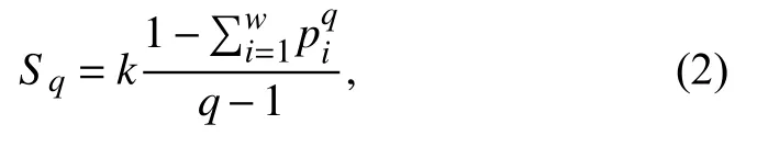
wherekis the Boltzmann constant,piis the probability that the system is in thei-th microstate andqis called the nonextensivity index,which characterizes the system and converges to unity in an equilibrium situation (so the Boltzmann entropy of a system is defined only if it is in physical thermodynamic equilibrium).Recently,this formalism was presented in a seismic context in Sotolongo-Costa and Posadas (2004).The idea is that,due to the rupture dynamics between tectonic blocks,material residues should fill the space between the faults.So,an increase in stress should be observed on the plates to overcome the resistance of fragments.Specifically,the non-extensive formalism was applied in the description of fragmentation,where Tsallis entropy is used to describe the transition into scaling.Here,the parameterqis related to an effective temperature of breakage,where long-range correlations should be raised significantly as the energy of breakage increases.Asqincreases from 1,the physical state goes away from equilibrium,what means that the surface along which there is slip during an earthquake is not in a physical equilibrium.The result is a model (which we will call the SP-model) for the energy distribution of earthquakes (and by them∝logErelation,for its corresponding frequency distribution of magnitudes) connected to the size distribution of fragments between the faults.Here,it will be shown that some of these models can be obtained alternatively under a Bayesian perspective,through a process of marginalization.

2.A Bayesian perspective

If we look inside the seismic context presented in Main et al.(2000),we findas a distribution consistent with percolation theory and statistical physics of critical pointphenomena,explaining locally the buildup and release of tectonic strain energy,where strain energy responds to external force from plate tectonics.But our previous informationIindicates that,in addition,there are actually a lotof other di_erent models presented by other authors explaining the observed statistical seismic behaviour (Anagnos and Kiremidjian,1988;Mignan,2015),so,wecan see that complexity of seismic process becomes evident [you can read about this issue in Chelidze(2017)].Then,in the light ofI,we suggest a generalization ofsuch as

Note that a function of the form (3) has already been used to explain observed seismic data (Wu MH et al.,2019).Here(E) is obtained as a particular case withδ=1.Now,we have a distribution for a scalar variableE,the energy released in the seismic activity,which depends on the parameterβ.For a discrete case of parameterβ,being able to take the valueβ1or the valueβ2,etc.,we have thatp(β1+β2+…|I)=1 (the Boolean operator "+" implies that one of propositionsβiis correct).The probability of the compound proposition is

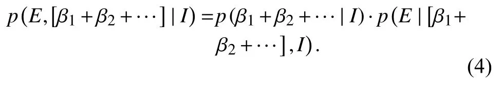
Usingtheproductrule and simplifying the expression for

Boolean algebra allows an expansion of the righthand side,and extending to the case whereβis a continuously variable parameter,we have the marginal posterior distribution forE,given by

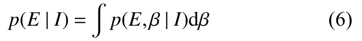
We don't know in advance the shape of the marginalp(β|I) related to the joint probabilityp(E,β|I),so it should be also determined based on our most recent knowledge update.In the literature we find that a Gamma distribution has a good performance in seismic applications through a Bayesian perspective (see,for example,Stavrakakis and Tselentis,1987;Galanis et al.,2002;Campbell,1982;Parvez,2007).Here,for the marginal,we also choose a more general form

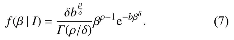
So,with (6) we obtain

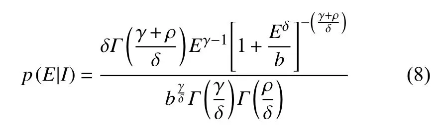
forE ≥ 0,γ ＞ 0,ρ ＞ 0,δ ＞ 0,b ＞ 0.This marginalization incorporates the uncertainty associated to the assignment of a specifi c value to the parameterβ,as well as the intrinsic uncertainty present inthe context of our specific problem.Here we see both,g(E|β) andf(β|I) in the generalized gamma family of functions.

3.Emergence of some non-extensive seismic models

3.1.Some current non-extensive models

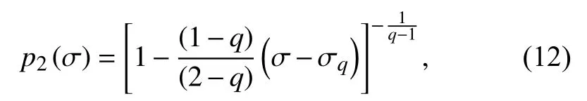
As you can see in Section 1,a non-extensive model(the SP-model) for frequency distribution of seismic magnitudes was presented.There,authors thought about the different fragments of material filling the gaps between the interacting tectonic plates which generate seismic activity.Then,through the Tsallis formalism,a probability function of finding a fragment with specific surface sizeσwas obtained,resulting in theq-exponential distribution for the fragment size

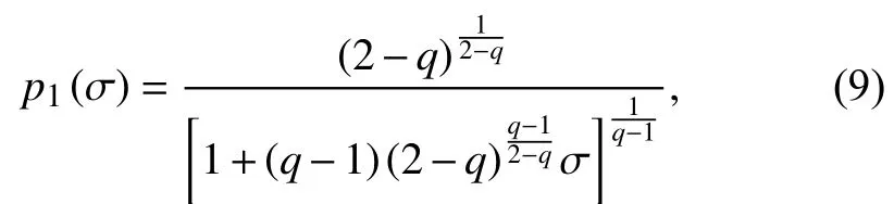
whereqis the non-extensivity parameter (which leads us to the Boltzmann statistic whenq→1).The seismic energyEdistribution,is obtained assuming

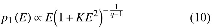
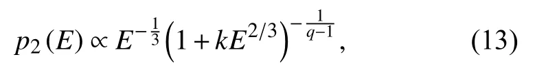
On the other hand,in Silva et al.(2006) a different choice of constraints for maximizing the non-extensive entropy led to the following fragment size distribution:

where,again,qis the non-extensivity parameter,whereq≠1(and some papers,as Silva and Lima (2005),indicate that it lies on the open interval [0,2]).Here,the choiceE∝σ3/2leads to the emergence of a different seismic energy distribution function,

3.2.Extended family of non-extensive distributions

We can get both of the non-extensive models from the caseγ=δin equation (8),that is,from

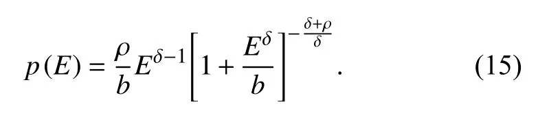
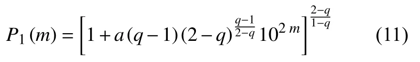
So,models given by equations (10) and (13)correspond to casesδ=2 andδ=2/3 respectively in equation (15).In this perspective,we have that

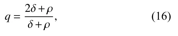
where constraints given forδandρin equation (8) lead us to 1 ＜q＜ 2 (see Figure 1).

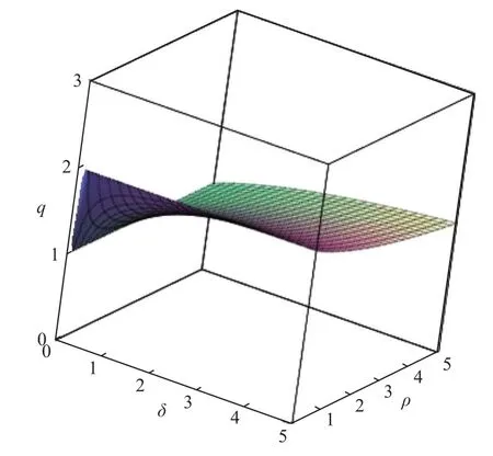
Figure 1.q parameter dependence,for ρ ＞ 0 and δ ＞ 0.

Figure 2.The three earthquakes selected for application of the model (17) to corresponding observed data.(Image taken from Map data ©2021 Google).

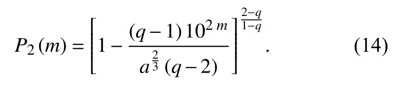
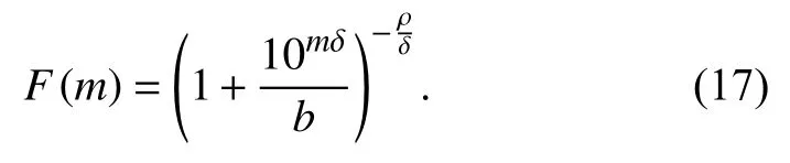
It seems that the relationship between the energy released from the earthquake and the size of fragments is something that could lead us to suggest new models.Quoting Sotolongo-Costa and Posadas (2004),about the SP-model,“No ad hoc hypotheses were introduced except the proportionality of E and r,which seems justified,....This is the simplest model that we can make,since in this representation a proportionality of the energy can be introduced with another power of r”.The above should allow us to pick aE∝σ1/δassumption.So,we also can take them∝logErelation in equation (15) to obtain the cumulative frequency-magnitude distribution

3.2.1 Application

At first glance,we might think that a non-fixed parameterδin equation (15) could explain different seismic behaviours observed in different geographical regions,while the other models could be limited due to the fixed value of said parameter.To test this,all the events reported in the Centro Sismológico Nacional de la Universidad de Chile (CSN) catalogue,for one month before and one month after three strong earthquakes ocurred in different regions (see Fig.2) were considered,

· Cauquenes 2010 (36.290° S,73.239° W),8.8 magnitude,February 27,2010

· Iquique 2014 (19.63° S,70.86° W),8.2 magnitude,April 01,2014

· Coquimbo 2015 (31.535° S,71.919° W),8.4 magnitude,September 16,2015

So,a set of six data samples was obtained.Each data sample contains local Richter magnitudes (ML) recorded in the entire territory of Chile during a month previous to the main event and,on the other hand,the magnitudes recorded during a month after the main event,including it(moment magnitude (MW) was taken whenMLmagnitude was not available).In this way,for the period between January 27,2010 and February 27,2010 (before the Cauquenes 2010 main event),we found 166 earthquakes in the CSN catalogue,with the minimum magnitude beingmmin=2.3 and the maximum magnitudemmax=6.4.Also,in the period between February 27,2010 (from the main event) and March 27,2010 we found 1 687 earthquakes,withmmin=2.5 andmmax=8.8.On the other hand,for the period between March 1,2014 and April 1,2014 (before the Iquique 2014 main event) we found 945 earthquakes,withmmin=2.5 andmmax=6.7.Futhermore,in the period between April 1,2014 (from the main event) and May 1,2014 there are 1 458 earthquakes recorded,withmmin=2.5 andmmax=8.2.And finally,during the period between August 16,2015 and September 16,2015 (before the main event of Coquimbo 2015) we have 362 earthquakes,withmmin=2.5 andmmax=6.0.Also,in the period between September 16,2015 (from the main event) and October 16,2015 we found 1 797 earthquakes,withmmin=2.5 andmmax=8.4.It should be noted that some papers show that small earthquakes provide relevant information on the seismic process,allowing to learn about the seismotectonics of the observed region (Ebel,2008),and we just have that,in the early stage of an aftershock sequence,small events may be missing from the catalogue.Missing data could affect certain types of analysis (Kagan,2004)but we want to know how our model behaves in this situation.So,the cumulative normalized distribution equation (17) was fitted to each of the data samples,as it can be seen in Figure 3,in order to check the ability of our expression to fit the data,sinceδis a free parameter.Simultaneously,equations (11) and (14) (both cases with a specific value for theδparameter in the perspective of our model) were applied to the same data samples for comparison purposes (their fit curves are not shown here,but they roughly overlap the plotted one).

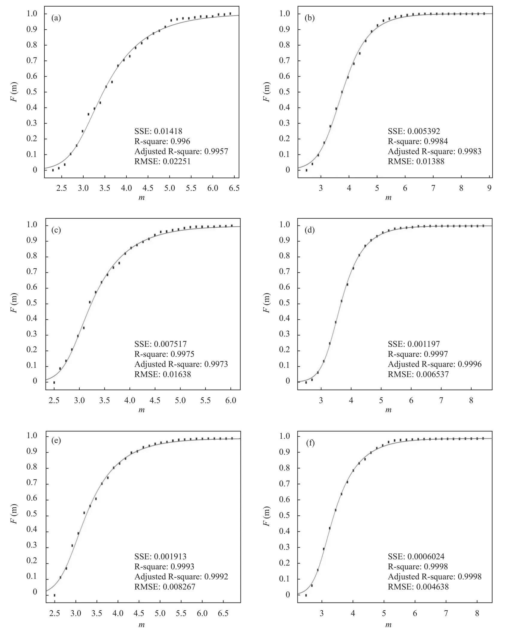
Figure 3.Fitted curve obtained with model (17) before (a) and after (b) of the main 2010 Cauquenes earthquake is shown.The same in (c) and (d) for the case before and after the 2015 Coquimbo earthquake,correspondingly,and for the case of Iquique 2014,in (e) and (f).Goodness of fit was inserted into each panel (sum of squared errors SSE,R-square,adjusted Rsquared and the root mean square deviation RMSE).

A summary of the fit parameters obtained through the nonlinear least squares (curve fitting) for all the models can be seen in Table 1.No exclusion was used to select the final dataset ,therefore,magnitudes less than the magnitude of completeness mc of the catalog,which the GR law has shown not be able to cover,were considered(an issue that can be seen in some papers where new models have been presented,such as Darooneh and Mehri(2010),Silva et al.(2006) and Sotolongo-Costa and Posadas (2004).) We can also readly see that,from the cumulative distribution corresponding to Equation (15),the well known power law scalingN(＞E)～E-Bcan be obtained.

Additionally,for comparison purposes,the GR relation and the model (17) are shown in Figure 4 for the seismic data belonging to the 2015 Coquimbo (after) event (which was already shown in Figure 3).Applying the GR model it is obtained that the value ofbis 0.808 5,while the value ofais 2.725.Usually,the Gutenberg-Richter cumulative frequency-magnitude law is used for assessing comp-leteness of an earthquake catalogue.(In Ruiz et al.(2016),about the seismic sequence of Coquimbo 2015 earthquake,it was determined that the CSN catalog for the Coquimbo region is complete fromML～ 4.0).

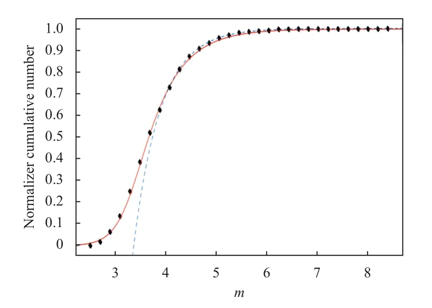
Figure 4.Cumulative distribution versus magnitude for Coquimbo 2015 seismic data (black diamonds),our model (17)(red solid line) and the GR law (blue dashed line).

4.Remarks

We have shown an alternative way that leads us to energy distributions of earthquakes (and hence to frequency distributions of magnitudes) known in the literature and based on non-extensive formalism,thus evidencing the relevance of these distributions in the explanation of the observed data.Also,we have that our model could be useful to explain data that,eventually,some known non-extensive models couldn’t.

We then wonder if we need to extend the known family of non-extensive distributions,that is,if distributions built by other authors (expressions (11) and(14),for example) are enough to explain the different data sets that may arise in different seismic events.This is equivalent to asking if our model can work satisfactorily with a fixed specificδparameter.Apparently,there would be no reason to think that there should be a single value forδ.

Looking at the seismic context,it seems reasonable to us to think that each geographical area,and its corresponding sub-soil structure,seismically responds according to its different configurations and specific failure mechanisms that controls the magnitude of stress at a particular time and place in the lithosphere (Engelder,1993).Therefore,opting for a free parameterδcould be a fair decision,because this might allow an adaptation of the model to different regions,according to local characteristics.However,when model (17) was applied to six different data samples,it has been found that its fit parameters show values that suggest a convergence towards the SP model.This can be seen in the summary presented in Table 1,where we get a same value for parameterqin both models (11) and (14),very close to the one obtained with our model (17),through equation (16).

On the other hand,when verifying the resulting value ofδparameter for each of chosen samples,it can be seen that it is much closer to theδ=2value,that characterizes the SP model.In fact,if we take an average ofδvalues obtained for all the data samples with (17),it is verified that=1.914.

Note that,on the other hand,this work could be a motivation to exhaustively explore a physical framework that takes into account the relevance,or not,of expression(15),considering that the Bayesian perspective used here and the expression obtained from it,have already been related to some physical formalisms known in the literature (see,for example Lavenda,1995;Beck and Cohen,2003;Mathai and Haubold,2011;Sattin,2006;Umpierrez and Davis,2021).