A comparative study of seismic tomography models of the Chinese continental lithosphere

Xuezhen Zhang ,Xiaodong Song,✉ and Jiangtao Li

1 Hebei Hongshan National Observatory on Thick Sediments and Seismic Hazards, Beijing 100871, China

2 School of Earth and Space Sciences, Peking University, Beijing 100871, China

3 School of Geodesy and Geomatics, Wuhan University, Wuhan 430079, China

ABSTRACT The Chinese mainland is subject to complicated plate interactions that give rise to its complex structure and tectonics.While several seismic velocity models have been developed for the Chinese mainland,apparent discrepancies exist and,so far,little effort has been made to evaluate their reliability and consistency.Such evaluations are important not only for the application and interpretation of model results but also for future model improvement.To address this problem,here we compare five published shear-wave velocity models with a focus on model consistency.The five models were derived from different datasets and methods (i.e.,body waves,surface waves from earthquakes,surface waves from noise interferometry,and full waves) and interpolated into uniform horizontal grids (0.5° × 0.5°) with vertical sampling points at 5 km,10 km,and then 20 km intervals to a depth of 160 km below the surface,from which we constructed an averaged model (AM) as a common reference for comparative study.We compare both the absolute velocity values and perturbation patterns of these models.Our comparisons show that the models have large (＞ 4%) differences in absolute values,and these differences are independent of data coverage and model resolution.The perturbation patterns of the models also show large differences,although some of the models show a high degree of consistency within certain depth ranges.The observed inconsistencies may reflect limited model resolution but,more importantly,systematic differences in the datasets and methods employed.Thus,despite several seismic models being published for this region,there is significant room for improvement.In particular,the inconsistencies in both data and methodologies need to be resolved in future research.Finally,we constructed a merged model (ChinaM-S1.0) that incorporates the more robust features of the five published models.As the existing models are constrained by different datasets and methods,the merged model serves as a new type of reference model that incorporates the common features from the joint datasets and methods for the shear-wave velocity structure of the Chinese mainland lithosphere.

Keywords: Chinese mainland;shear-wave velocity model;model comparison;continental lithosphere.

1.Introduction

The Chinese mainland is located in the southeast of the Eurasian Plate at its intersection with the Pacific Plate and the Indian Plate.This region has a very complex geological background with intricate interactions among many blocks and orogenic belts including the North China Craton in the north,the Precambrian Yangtze Craton in the south,the Tarim Craton in the northwest,the Qinling Orogenic Belt in the central area,and the Tibet-Himalayan Orogenic Belt in the southwest (Figure 1).Such complex tectonics makes the area–particularly western China–one of the most seismically active regions in the world.

Seismic tomography models are key to understanding the interior structure of the Earth and regional tectonics.In the past few decades,the increase in the number of seismic stations in China’s national and regional networks has led to a substantial increase in the availability of seismic observation data (Figure 1).This has enabled the construction of high-resolution velocity models of the lithosphere of the Chinese mainland.Indeed,in recent years,many studies have developed shear-wave (S-wave) velocity models based on various methods including ambient noise and earthquake surface-wave tomography (Yang YJ et al.,2012;Li YH et al.,2013;Bao XW et al.,2015;Shen WS et al.,2016;Yang ZG and Song XD,2019;Peng J et al.,2020;Witek et al.,2021;Li MK et al.,2022),body wave tomography (Wei W et al.,2016;Xin HL et al.,2019;Wei W and Zhao DP,2020),full waveform inversion (Chen M et al.,2015;Tao K et al.,2018),and joint inversion (Chen YL and Niu FL,2016;Han SC et al.,2022;Xiao X et al.,2021).Despite the availability of these models,there has been no comprehensive evaluation of their consistency;while each model may provide the optimal fit for the particular dataset used,their consistency has not been evaluated.The differences and the robustness of models are important as these indicate the overall reliability of model outputs as well as their applicability and interpretation by both model researchers and tomography users.Moreover,evaluations of model performance and consistency can guide their future improvement.

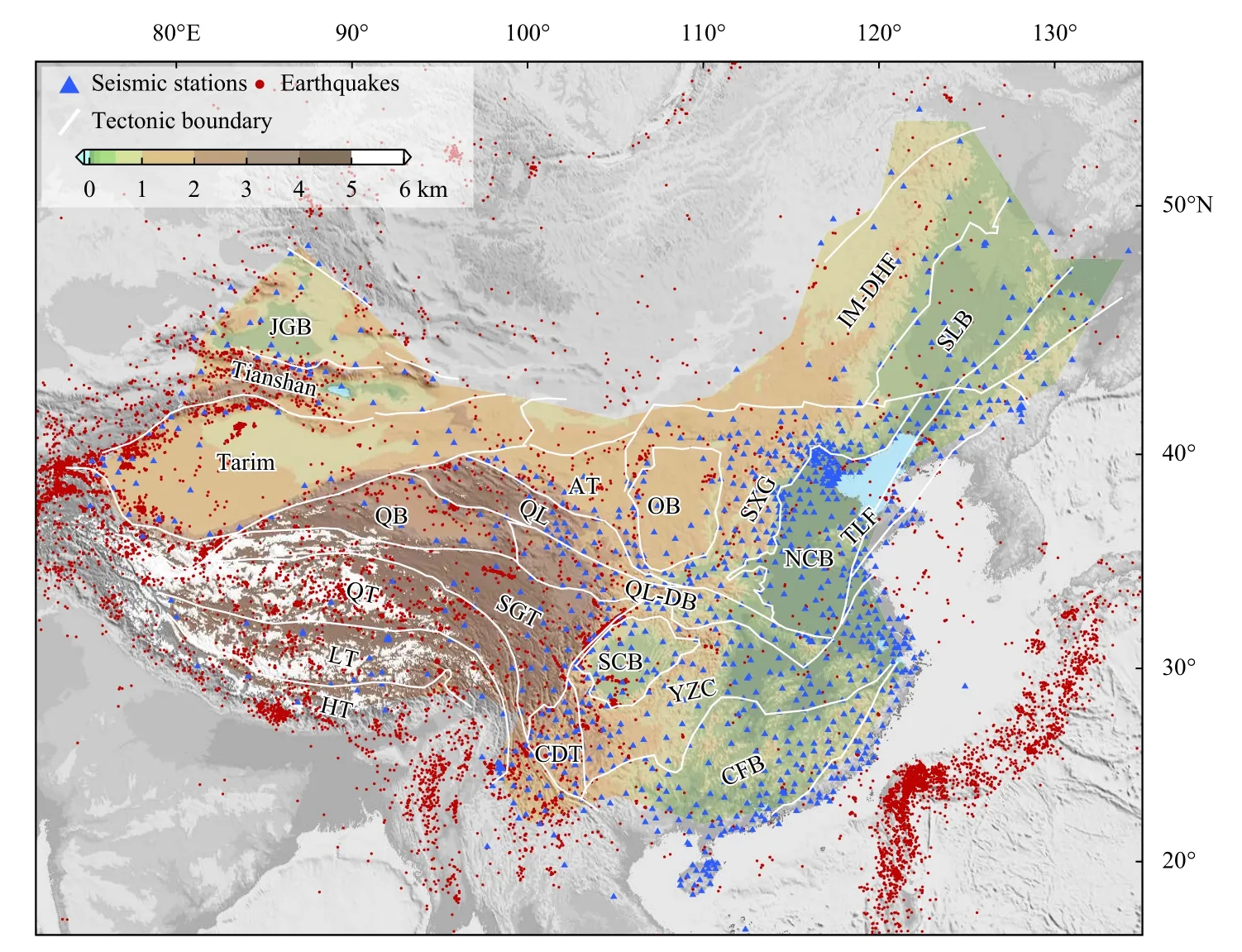
Figure 1.Main blocks and tectonic units of the Chinese mainland (modified from Liang CT et al.,2004;Xin HL et al.,2019) showing the distribution of China national and regional seismic networks (blue triangles) and earthquakes (red dots,magnitude ＞ 3,depth ＜ 150 km) recorded between 2000 and 2020.The area shown in color indicates the study area.JGB:Junggar Basin;QB: Qaidam Basin;QT: Qiangtang Terrain;LT: Lhasa Terrain;HT: Himalayan Terrain;SGT: Songpan-Ganzi Terrain;CDT: Chuandian Terrain;SCB: Sichuan Basin;QL-DB: Qinling-Dabie Orogenic Belt;QL: Qilian Orogenic Belt;AT: Alashan Terrane;OB: Ordos Terrane;SXG: Shanxi Graben;YZC: Yangtze Craton;CFB: Cathaysia Fold Belt;NCB:North China Basin;TLF: Tanlu Fault;SLB: Songliao Basin;IM-DHF: Inner Mongolia-Daxinganling Fold Belt.

Therefore,in this study,we specifically aim to address this need by evaluating the degree of consistency among a range of seismic models of the Chinese continent.Furthermore,based on the mutual consistency of the models,we constructed a merged model (ChinaM-S1.0) to serve as a new type of reference model containing the more robust features of different models of the S-wave velocity structure of the Chinese mainland lithosphere.It should be noted that we only sought to analyze the consistencies,similarities,and differences among the selected models and do not directly judge which model is better or worse.Based on our comparisons,we were able to determine whether the inverted S-wave velocity models were consistent,analyze the differences among them,and identify the possible causes of these differences.

2.Data and methods

2.1.Original models

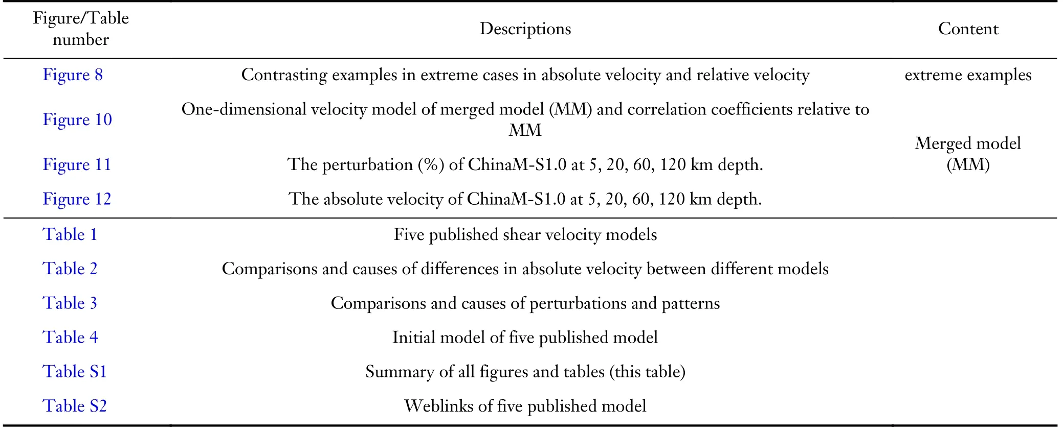
We screened a series of published S-wave velocity models of the lithosphere of the Chinese mainland along with the data and methods used (Table 1).Witek et al.’s(2021) model (accounting for anisotropy) was not considered,as we found that the model data did not match the figures in the paper.In total,we selected five published S-velocity models (Table 1;Figure 2;Figures S1–S3),referred to as ‘Li13’ (Li YH et al.,2013),‘Bao15’ (Bao XW et al.,2015),‘Shen16’ (Shen WS et al.,2016),‘Xin19’ (Xin HL et al.,2019;USTClitho1.0),and ‘Tao18’(Tao K et al.,2018),respectively.Although an updated model by Han SC et al.(USTClitho2.0,2022) is now available,which combines surface-wave data,we used the previous version (USTClitho1.0) based on body wave data to allow comparison using different data types.Similarly,although an updated model to Bao15 is now available (Li MK et al.,2022),we used the previous version as it is primarily based on ambient noise data,which enables the comparison of different data types (below);the updated Bao15 model (Li MK et al.,2022) includes more earthquake data.Our analyses generated many figures;therefore,we have generally chosen to present representative plots in the main text and reserve others for the Supplementary information.For the convenience of crossreferencing,we list all the figures and tables in Table S1.

We re-interpolated the velocity models in uniform grids at the same depth,latitude,and longitude.The horizontal interpolation interval was 0.5° × 0.5°,and the vertical interpolation intervals were 5 km,10 km,and then increasing to 20 km for the depth range 40–160 km.Thus,we focused on crustal and lithospheric mantle structure(Figure 2 and Figures S1–S3).The original grid size of the Bao15,Shen16,and Xin19 models was 0.5° × 0.5°,and that of Tao18 was 0.25° × 0.25°,which satisfied our horizontal sampling.The Bao15,Tao18,and Xin19 models were also sampled at depths that satisfied our vertical sampling,meaning there were no secondary changes made to these three models.The Li13 model was reinterpolated from its original 1° × 1° grid resolution.Forthe sake of brevity,we only provide comparative results for 5,20,60,and 120 km depths,which is sufficient to show the distinct features of the models.All model data sources are listed in Table S2.Plots of the five models at the selected depths (i.e.,5,20,60,and 120 km) are shown in Figure 2 and Figures S1–S3.

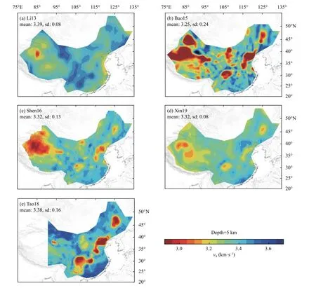
Figure 2.Five published shear-velocity models (a–e,see Table 1) at a 5 km depth with the same color palette.The onedimensional mean velocity (km/s) and standard deviation (sd) are labeled.Other depths are shown in Figures S1–S3.

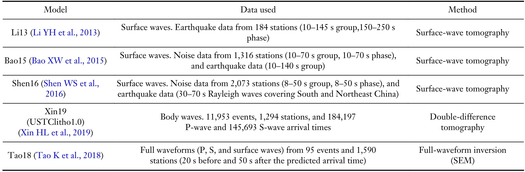
Table 1.Five tomographic models compared in this study.

2.2.Averaged model (AM)

From the five original models,we defined an averaged model (AM) using the same uniform grid with its main boundary close to the outline of the Chinese mainland(Figure 1).The AM represents an average of the five models with some detailed considerations.For each grid point inside the AM boundary,the input model values were combined to derive the AM value.If a model did not have a value at that point,it was not used;if there was only one model value among the five models,this was used as the AM value.The AM provides a common baseline,i.e.,a reference model,to evaluate the consistency of the five models.

2.3.Model evaluation

2.3.1 Absolute velocity

To evaluate the absolute velocity results of the models,we examined the difference between each model and the AM values at each grid point,as follows:

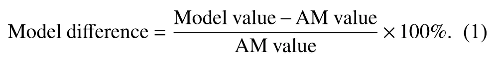
The mean and standard deviation (SD) of the model difference (Equation 1) at all grid points of each depth were also calculated.

2.3.2 Perturbation patterns

As perturbations better reflect lateral variations and three-dimensional (3D) model structures,most previous studies have focused on model perturbations,i.e.,the difference of each grid point at a given depth relative to a one-dimensional (1D) average velocity at that depth,rather than absolute velocity differences.While four of the models covered the entire study area,Tao18 did not.Therefore,to compare the perturbations between the models using the same color pallet,a baseline shift was applied to the velocity perturbations of the Tao18 model.This was applied relative to the average of the region covered by the model (i.e.,central and eastern China) by adding the average value of the AM for the same region.

We used two methods to quantify the similarity and consistency of each model’s perturbations.First,the correlation coefficient (CC) between two models was defined as follows:

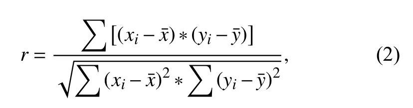
wherexandyare the perturbations of the two models,andxiandyiare the perturbation values of the two models at the grid pointi.The symbolsor are averages of all grid points at the given depth forxory,respectively.This coefficient was used to judge the similarity between the perturbation patterns of each pair of models.

Second,the difference between the perturbations of each model and the AM at each grid of a given depth was calculated as follows:

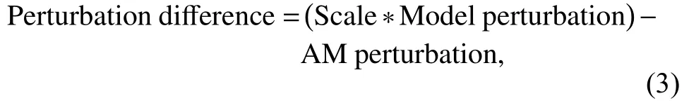
where ‘Scale’ is the scaling factor of the model perturbations for the given depth.We determined the scaling factor using the least-squares method by minimizing the variance of the perturbation differences of all the grids at that depth after scaling.The perturbation differences also reflect the similarity of the patterns in different grids.In addition,we determined the SD of the model differences for all the grids of the given depth,and judged the similarity of the overall patterns.The scaling factor reflected the amplitude of the model perturbations,where a smaller scaling factor (＜ 1) indicates that a model’s perturbation amplitude was larger than that of the AM,and vice versa.For example,assuming that the pattern of a model’s perturbations is very similar to the pattern of the AM perturbations,and the perturbation amplitude is twice the AM perturbation amplitude,the CC (Equation 2) will be close to 1 while the scaling factor (Equation 3) will be close to 0.5.After the scaling,the perturbation difference in each grid,and the SD of the perturbation differences in all grids,will be close to zero.

3.Results

3.1.Averaged model (AM)

The AM is shown in Figure 3 and Figures S4–S6 for selected depths.We also calculated the AM velocity perturbations (relative to the average at that depth) and the model error of the AM,defined as two SDs of the five models at a given grid point.The AM,representing the average of the five original models,shows well-known overall features of the Chinese mainland lithosphere(Figure 3a and Figures S4a,S5a,and S6a).In the upper and middle crust,the sedimentary basins in China,including the North China,Songliao,Tarim,Jungar,and Sichuan Basins,show conspicuous low-velocity anomalies.A low-velocity zone also appears in the Tibetan Plateau region.In contrast,the eastern Chinese mainland shows relatively high velocities (Figure S4a).In the lower crust,a prominent low-velocity anomaly is seen beneath Tibet.In the uppermost mantle,the cratonic roots beneath the Tarim,Ordos,and Sichuan Basins are shown as highvelocity anomalies.Based on the error distribution maps of the AM,we found large differences in absolute velocity (＞4%) between the models in most areas at shallower depths(5–60 km) (Figure 3 and Figures S4 and S5),while these differences were less notable at greater depths (120 km;Figure S6).

3.2.Absolute velocity

In this section,we focus on comparing the absolute velocities of the models using the AM as a common reference.We calculated averaged 1D velocity profiles for all six models (Figure 4) for the common region covered by Tao18 only,providing the same basis for comparison.Refer to Table S1 for the indices of the relevant figures regarding absolute velocity.

3.2.1 Model consistency in absolute velocity

The overall trends of the 1D velocity models with depth are quite similar (Figure 4a).At depths greater than 60 km(e.g.,Figure.S6d at 120 km),the errors of the AM (2 × SD of the five models at each grid) are less than 4% in most areas,while there are more areas with high errors at shallower depths (Figure 3 and Figures S4 and S5).This indicates better agreement in the absolute velocities of the models for the uppermost mantle.

3.2.2 Model inconsistency in absolute velocity

Relative to their consistent features in absolute velocity,inconsistencies among the models were notably more pronounced.For the 1D models (Figure 4),although the overall trends are similar,the models still diverge significantly,and the SDs of the models relative to the AM vary by up to 3% at all depths (Figure 4b).More importantly,some models are systematically fast (e.g.,Tao18 at all depths) and some are systematically slow (e.g.,Bao15 at all depths).

Figure 3.Averaged velocity model (AM) perturbations and error at 5 km depth.Model error is defined as two standard deviations (SDs) of the velocity values of the five original models at each grid point (Table 1).(a) AM at 5 km depth (average velocity=3.3 ± 0.12 km/s with one SD,labeled as “sd”);(b) Error distribution of (d) shown as a percentage histogram;(c) Map of perturbations of the AM based on 1D averaged velocity (SD of the perturbations is labeled,in percent);(d) Map of the AM errors.Additional depths are shown in Figures S4–S6.

Such systematic differences are also clear in the map views.For example,at 20 km (Figure 5),almost all regions of the Bao19 model results are slower than in the AM (by 4% on average),while most regions in the Xin19 and Li13 results are faster than in the AM (by 3% and 2%,respectively,on average).Similar systematic differences are also be observed at other depths (Figures S7–S9).

3.3.Relative velocity

We compared the relative velocities of the models in the following two ways: (1) velocity perturbation patterns(relative to each model’s average velocity at a given depth)and CCs between the model perturbations (Figure 6 and Figures S10–S12);and (2) the model difference between the scaled perturbations and the AM perturbations (Figure 7 and Figures S13–15).The CCs between each model and the AM with depth are also shown in Figure 4c.In most previous studies,greater attention has been given to the overall patterns of models rather than to absolute velocities,which better show lateral variations.Thus,here we focus on the pattern consistencies and inconsistencies of the models.

3.3.1 Model consistency in perturbation patterns

Generally,the individual models show good agreement with respect to perturbation patterns and major geological features at different depths.At shallower depths (5–20 km,Figure 6 and Figure S10),pronounced low-velocity perturbations (amplitude ＞ 6%) exist beneath the large sedimentary basins (i.e.,the Tarim,Sichuan,Songliao,and North China Basins) and the Tibetan Plateau.Close to the upper mantle,the main low-velocity zones appear in the Tibetan Plateau region,while high velocities are present in the east along with large perturbation amplitudes in all of the models (Figures S10–12).In the uppermost mantle(120 km,Figure S12),the Sichuan Basin,the Ordos Block,and the Tarim Block all show high-velocity perturbations(up to 6%),while the central Tibetan Plateau shows a relatively low-velocity anomaly,and the whole of eastern China also shows relatively low velocities.

：“，，。I didn`t feel that I had anyone to say those words to, and besides,，，who were you to tell me to do something that personal8?？？“But as I began driving home my conscience2 started talking to me

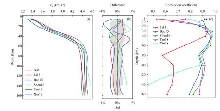
Figure 4.One-dimensional (1D) velocity model results of the five original models,and correlation coefficients relative to the averaged model (AM): (a) absolute 1D averaged velocities of each model (for the Tao18 model region,see Table 1);(b) Difference (%) between the original models and the AM (the grey region shows ± one SD of the 1D velocity profiles of the original models);(c) Correlation coefficients (CCs) between each model and the AM with depth.Note that we interpolated Li13 from the original 1.0° × 1.0° horizontal grid to 0.5° × 0.5°,although this only had a very small effect on the CC because very little of the overall pattern in horizontal perturbations was changed.

The CCs of most models (except Li13) with the AM are relatively high within the 20–100 km range (Figure 4c).In particular,the CCs of the Bao15,Shen16,Tao18,and Xin19 models with AM exceed 0.85 within this depth range,and show good agreement with each other at all depths except very shallow depths (5 km).Good agreement was also observed between all models except Li13 at the example depths of 20 and 60 km (Figures S10 and S11).

3.3.2 Model inconsistency in perturbation pattern

The inconsistency between some of the models is clear in the 1D CC profiles with the AM (Figure 4c).The CCs for Li13 are low at most depths,and those for Xin18 are also low at depths ＞ 100 km.The CCs for shallow depths(5 and 10 km) diverge greatly;they are low for Li13,Tao18,and Xin18.

In the map views and the mutual model correlations,most CCs are below 0.7 at 5 km (Figure 6) and 120 km(Figure S12) depths;at intermediate depths (20 km,Figure S10;60 km,Figure S11),the CCs are better except for Li13.In the maps of perturbation differences at different depths (Figure 7 and Figures S13–S15),the largest values are scattered across different areas.The largest departures from the AM are a 2.2% SD at 5 km(Xin19),1.6% at 20 km (Bao15),1.5% at 60 km (Bao15),and 1.3% at 120 km (Xin19),respectively,even after the application of scaling (i.e.,focusing only on the patterns)and excluding Li13,which has systematic differences and larger values.Compared with the SD of the AM perturbations at these depths (3.5%,3.3%,4.3%,and 1.7%at 5,20,60,and 120 km depths,respectively) (Figure 3 and Figures S4–S6),these values are significant.

4.Discussion

We compared five published S-wave models of the Chinese mainland and derived an averaged model (AM) of absolute velocity and perturbation patterns.Our results show that there are significant differences between these models,although there are also some consistencies.Figure 8 shows comparisons of extreme cases.The absolute velocity difference between Bao15 and Xin19 at 100 km averaged 2.0%,while the CC (Figure 6f) between the perturbation patterns of Tao18 and Li13 was close to zero(-0.07).The causes for these differences include a variety of factors,including different types and sources of data,inversion methods,initial models,and inversion parameters.We summarize the main differences identified in the following sections,and discuss their possible causes.

Figure 5.Model difference in absolute velocity at 20 km depth relative to the averaged model (AM) (Equation 1).(a–e)Differences (%) in absolute velocity values for each model (Table 1) are shown using the same color palette.The labels indicate the name of the model and the mean and SD of the differences.Other depths are shown in Figures S7–S9.

4.1.Absolute velocity

Differences in the absolute velocity and their possible causes are summarized in Table 2.Based on the velocity depth maps of four representative locations (the Tarim Basin,the Sichuan Basin,North China,and Tibet),large differences between the models can be observed at all locations (Figure 9).Some regions (e.g.,the Sichuan Basin and North China) have better ray coverages and higher resolutions,yet the differences are still as large as in other regions.This indicates that data coverage or model resolution may not be the most important factor explaining the model differences,although model results can vary widely depending on data resolution.

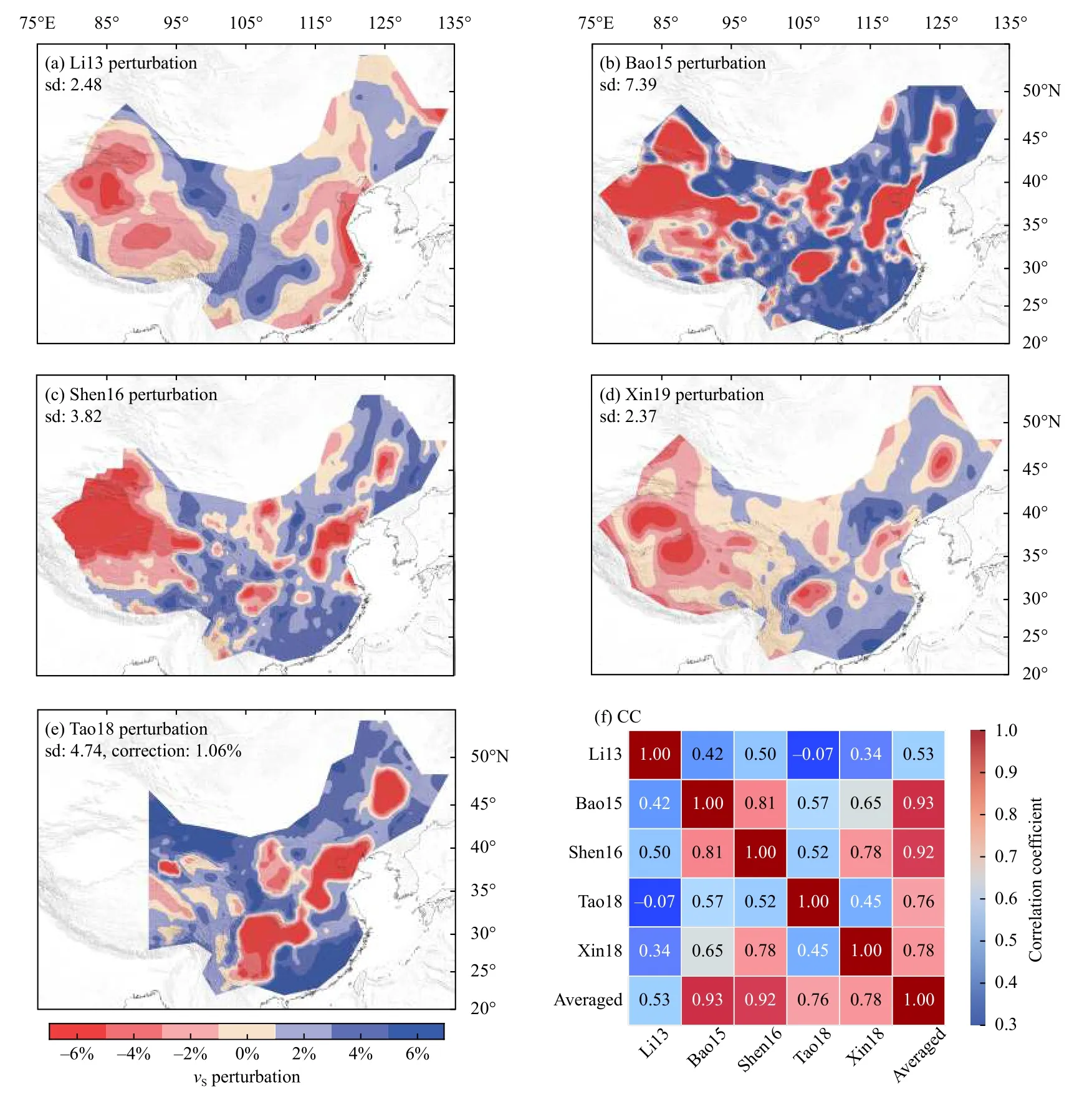
Figure 6.Model perturbations and correlation coefficients (CCs) of the models at a 5 km depth.(a–e) Velocity perturbation maps of the original five models (see Table 1) shown using the same color palette.The standards deviation (SD) (%) of the perturbations of each model at a particular depth is labeled.Note that the color scale of (e) is corrected according to the average perturbation value of the averaged model (AM) in the same region as the Tao18 model to enable comparison.(f) CC matrix of the models.The color and number of each grid indicate the corresponding CC between each model pair.Results for other depths are shown in Figures S10–S12.

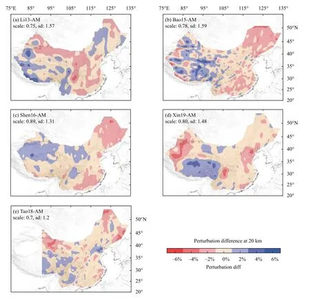
Figure 7.Maps of perturbation differences at 20 km depth relative to the averaged model (AM)(a–e).The same color palette is used for all the plots.The perturbation difference is defined in Equation 3 with the optimal scaling factor labeled for each model.The standard deviation (SD) of the perturbation differences for each model is also labeled (%).Results for other depths are shown in Figures S13–15.

Our analysis of the differences in absolute values shows that the Li13 model yields relatively faster (slower)velocities at a depth of above (below) approximately 60 km,which may be due to the difference in the dispersion curve measurements (from earthquake data) and inversion methods.On the other hand,the absolute velocities of the Bao15 model are systematically slower,which uses surfacewave dispersion curves from ambient noise more than those from earthquake data.Thus,one reason for the absolute velocity difference among the models might be systematic differences between data types (e.g.,earthquake vs.ambient noise).Indeed,Yao HJ et al.(2006,2008) note that the phase velocity acquired using the two-station method is higher than that acquired with ambient noise.In addition,we suspect different measurement and inversion methods will likely lead to differences in absolute velocity.

4.2.Relative velocity

Differences in the perturbation patterns of the models and their possible causes are summarized in Table 3.The following causes are particularly noteworthy: (1) as previously mentioned,differences in data types (i.e.,surface-wave dispersions from noise and earthquakes,body waves,and full waves) certainly play a role in the patterns of differences;(2) inversion parameters and methods may have an effect,including model damping,which is commonly used in tomographic inversions and affects model perturbations.From the optimal scaling factor used in the calculation of the perturbation differences (Equation 3),there is relatively large damping when the scaling factor is ＞ 1 (e.g.,Xin19 at depths ＜ 100 km and Li13 at depths ＞ 60 km) and relatively small damping when the scaling factor is ＜ 1 (e.g.,Bao15 and Shen16 at all depths);(3) inversion results may be affected by the choice of initial model (see Table 4).For Li13,the initial model contains discontinuities in the Moho and the crust,and such discontinuities may affect the final model,particularly when the initial model is used to dampen the inversion,which may artificially impose the assumed discontinuities;and (4) although the inconsistency in data types is critical,we also believe data coverage and model resolution could be important factors in some cases,e.g.,Xin19 at depths ＜ 10 km and ＞ 100 km.

4.3.Summary of the inconsistencies in the models and their causes

Difference features in each model and their possible causes are summarized in Table 2 and Table 3.The inversion problem for velocity structure is typically nonlinear and non-unique and,thus,the inversion results are subject to the effects of inversion methods and strategies.Furthermore,the 3D velocity structure of the Chinese continent is quite complex.Differences in data sampling will almost certainly result in variable results.In the following sections,we outline some important differences in the data and methods that may have contributed to the observed differences between the selected models.This is important for identifying potential controlling factors that can be targeted in the future refinement of these models.

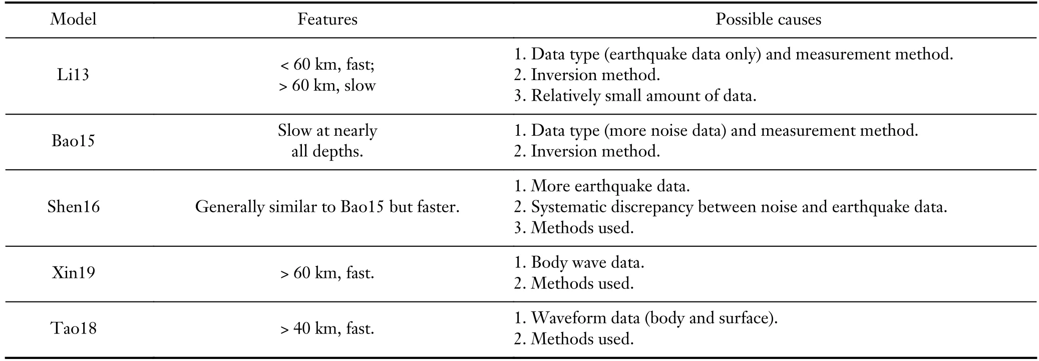
Table 2.Comparisons and causes of differences in absolute velocity.

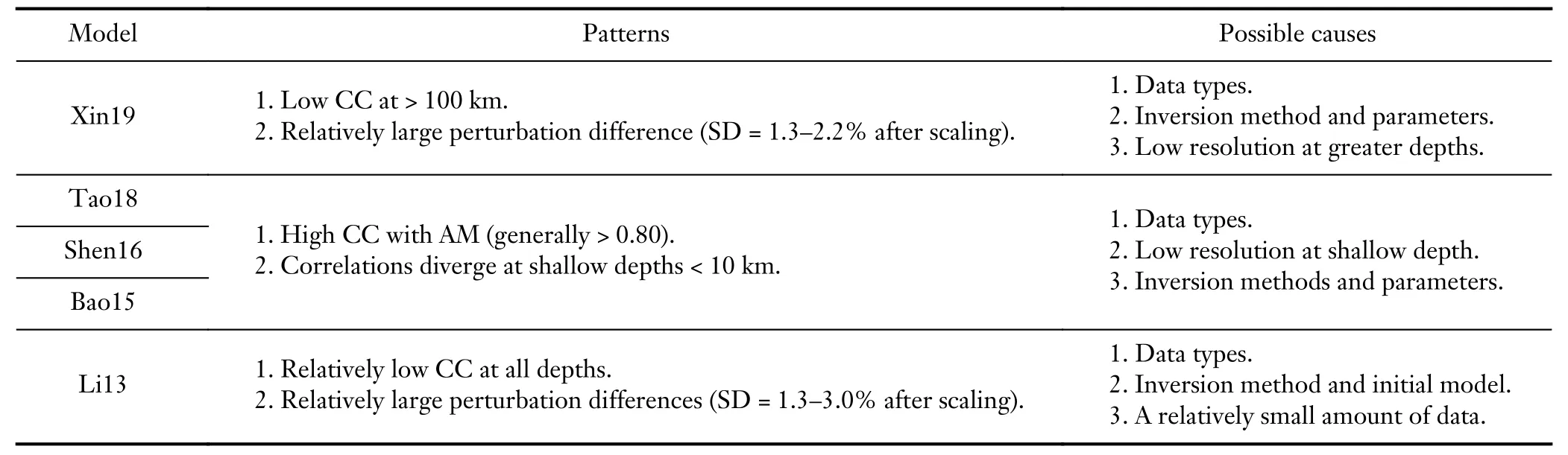
Table 3.Comparisons and causes of perturbations and patterns.

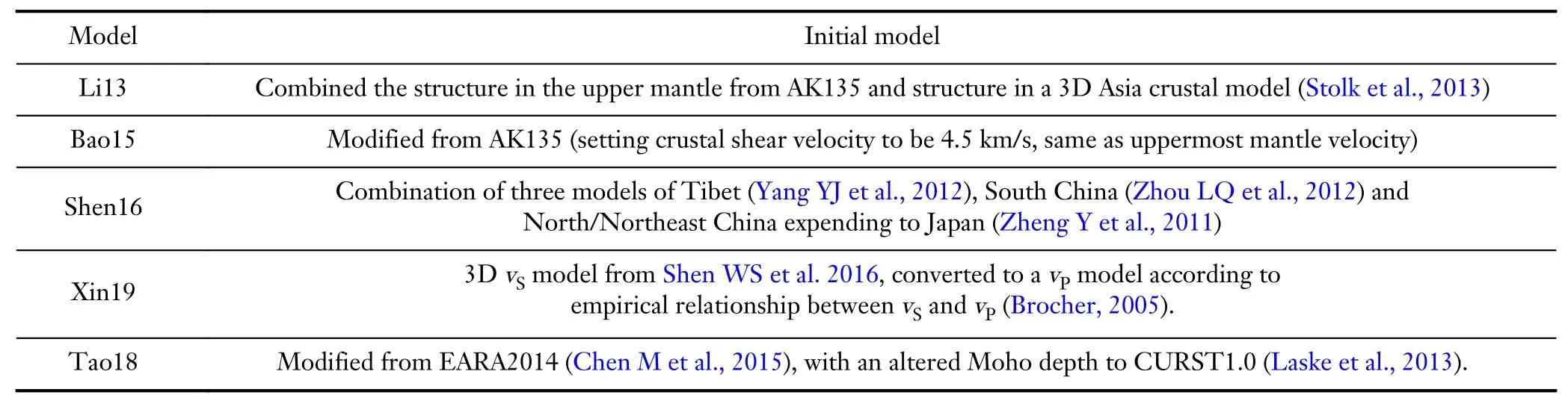
Table 4.Initial models for the five published shear-wave velocity models.

4.3.1 Data differences

First,data differences in the form of quantity differences (e.g.,the relatively small amount of data in the Li13 model) and data types or discrepancies in their sources,such as dispersion curves from ambient noise or earthquakes,can lead to variable results.In particular,for surface-wave tomography,the consistency between noise and earthquake data needs to be further verified.The velocity results obtained using noisier data may be lower,as reflected by the Bao15 model,which showed the slowest velocities compared to the other models.In addition,we found that the results obtained from the full waveform data and the surface-wave data were in good agreement.Data coverage may not be the dominant cause of model discrepancy,however,as we found differences even for locations with high data coverage (e.g.,the Sichuan Basin and North China;Figure 9).

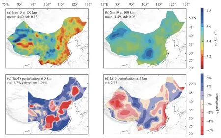
Figure 8.Contrasting velocity features derived from different velocity models for the Chinese mainland.(a) Bao15 model outputs at a 100 km depth,mean velocity=4.4 km/s;(b) Xin19 model outs at a 100 km depth,mean velocity=4.49 km/s.Note that (a) and (b) are drawn using the same color palette;(c) Tao18 model perturbations at a 5 km depth with 1%correction;(d) Li13 model perturbations at a 5 km depth.Note that (c) and (d) are drawn using the same color palette.

The differences at shallow depth (＜ 10 km) are large in absolute velocity and velocity perturbations among all the models.This is even true in the case of the perturbation patterns of the Bao15,Shen16,and Tao18 models,which have relatively high CCs at depths greater than 10 km but diverge greatly at shallow depths.The main cause of this is probably their lower resolution at shallow depths,which,in turn,is due to the lack of short-period (＜ 8 s) surfacewave data coverage and body-wave coverage.Note that in Figures 4 and 9,the 1D velocity difference of each model relative to the AM varies between the crustal and mantle depths.This is a good indication of the trade-off between the resolutions of the crustal and mantle structures.Such a trade-off is common in seismic tomography,such as in joint inversions of receiver functions and surface-wave dispersions (Li JT et al.,2017;Deng YF et al.,2018).

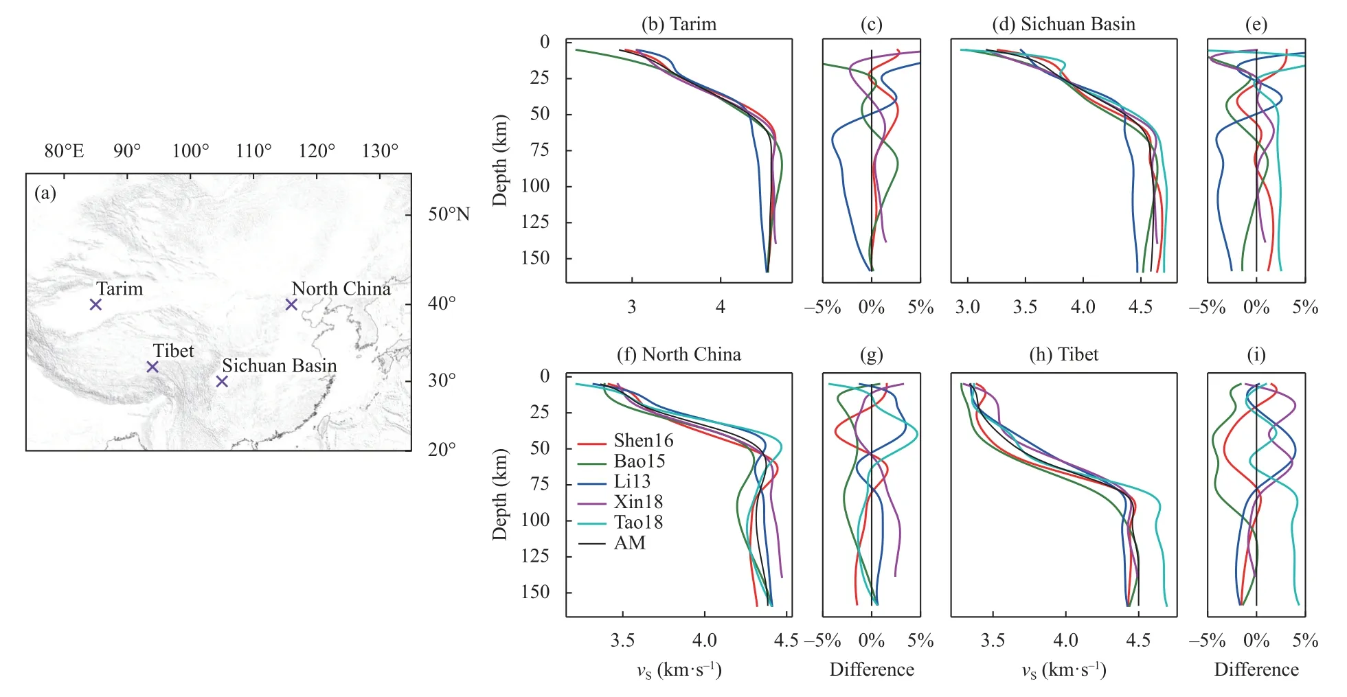
Figure 9.One-dimensional (1D) velocity models at selected locations (the Tarim Basin,Sichuan Basin,North China,and Tibet).(a) Locations of the 1D velocity models (purple crosses);(b) Tarim 1D velocity model and (c) its difference compared to the averaged model (AM);(d) Sichuan Basin 1D velocity model and (e) its difference compared to the AM;(f) North China 1D velocity model and (g) its difference compared to the AM;(h) Tibet 1D velocity model and (i) its difference compared to the AM.

4.3.2 Methodological differences

Different dispersion-curve measurement methods in surface-wave tomography analyses,different tomography methods,and different initial models also contribute to variations in model results.For example,in surface wave inversions,different inversion strategies have been used in the starting models (e.g.,Li13 and Bao15).The starting model of Li13 includes a crustal model with a Moho discontinuity;if the crustal thickness is not correct,it will bias the surface-wave inversion result.On the other hand,Bao15 assumes a starting model with a constant velocity of 4.5 km/s for the crust and mantle.The surface-wave inversion will smooth the Moho discontinuity,which tends to overestimate and underestimate the velocity directly above and below the Moho,respectively.

Furthermore,model parameters such as smoothing and damping during the inversion process also have an effect on the amplitude and overall pattern of results,as in the case of the Bao15 and Xin19 models,with relatively high and low amplitudes,respectively.

4.4.Merged model (MM)

Based on our analyses of model consistency and inconsistency,we selectively merged some of the models to obtain a new merged model (MM).The goal here was to generate a model that is consistent–to the greatest possible extent–with the component models.The 1D-averaged velocity model and perturbation model of the MM were obtained separately.

The merged model incorporates more robust features of the existing models that are constrained by different data sets and methods.Thus,the merged model is a better representation for common model features that fit the joint data sets than any of the individual model.This MM can serve as a new type of reference model for the S-wave velocity structure of the Chinese mainland lithosphere.As few studies have rigorously compared the performance of existing models,it is difficult to judge which individual model is better.Thus,the MM provides a useful reference model while a better or best model is identified based on rigorous evaluation.

4.4.1 Steps to construct the MM

First,based on the five original candidate models(Table 1),we calculated a 1D averaged model (1D MM0),which was then used to calculate a new 3D absolute velocity model together with the merged 3D perturbation model (Section 4.4.2).Second,we took an iterative approach to obtain the merged perturbation model.We defined the initial candidate perturbation models,which may or may not be the same as the initial candidate models for absolute velocity,and adopted the following procedure to obtain the new merged perturbation model: (1) calculate a merged 3D perturbation (MM0 perturbation model) from the initial candidate models following the same procedure as for the calculation of the AM outlined in Section 2.2;and (2) screen the initial candidate models and remove low-consistency models based on the CCs of their respective perturbations relative to the MM0 perturbation model(step 1) and re-calculate the perturbation model (MM1).These steps can be repeated as necessary,although we only performed one iteration in this study.Finally,we added the 1D MM0 model and the MM1 perturbation model at each depth to obtain a 3D model of absolute velocity,which we named ‘ChinaM-S1.0’.We also recalculated averages for each depth to obtain the 1D averaged model of the final merged model (i.e.,1D MM1 or 1D ChinaM-S1.0).

4.4.2 Initial 1D averaged model

For the initial candidate models,we excluded the Li13 model because of low CCs (Figure 4c),while the Xin19 model was only retained for the intermediate depth range(10–100 km) due to the lower resolution of body waves at shallow (＜ 10 km) and deep (＞ 100 km) depths.We retained the Bao15,Tao18,and Shen16 models at all depths.We averaged all of the retained models at the corresponding depths to obtain the 1D velocity profile of the initial merged model,MM0 (Figure 10a).

4.4.3 Screening of existing perturbation models and the construction of the MM

Due to the low CCs of the Li13 model (Figure 4c),we excluded this and defined the remaining four models (i.e.,Bao15,Shen16,Tao18,and Xin19;Table 1) as the initial candidate perturbation models to calculate the initial MM0 perturbation model.We then obtained the CCs between the candidate models and the MM0 perturbation model at different depths (Figure 10b).Xin19 showed lower CCs at depths of ＜ 10 km and ＞ 100 km,and Tao18 showed lower CCs at depths ＜ 20 km (all ＜ 0.82,appearing as clear outliers relative to those of the other models).Therefore,at the next iteration,the models with lower CCs were excluded at these corresponding depths.We then calculated the next perturbation model (MM1) with the remaining models at each depth.

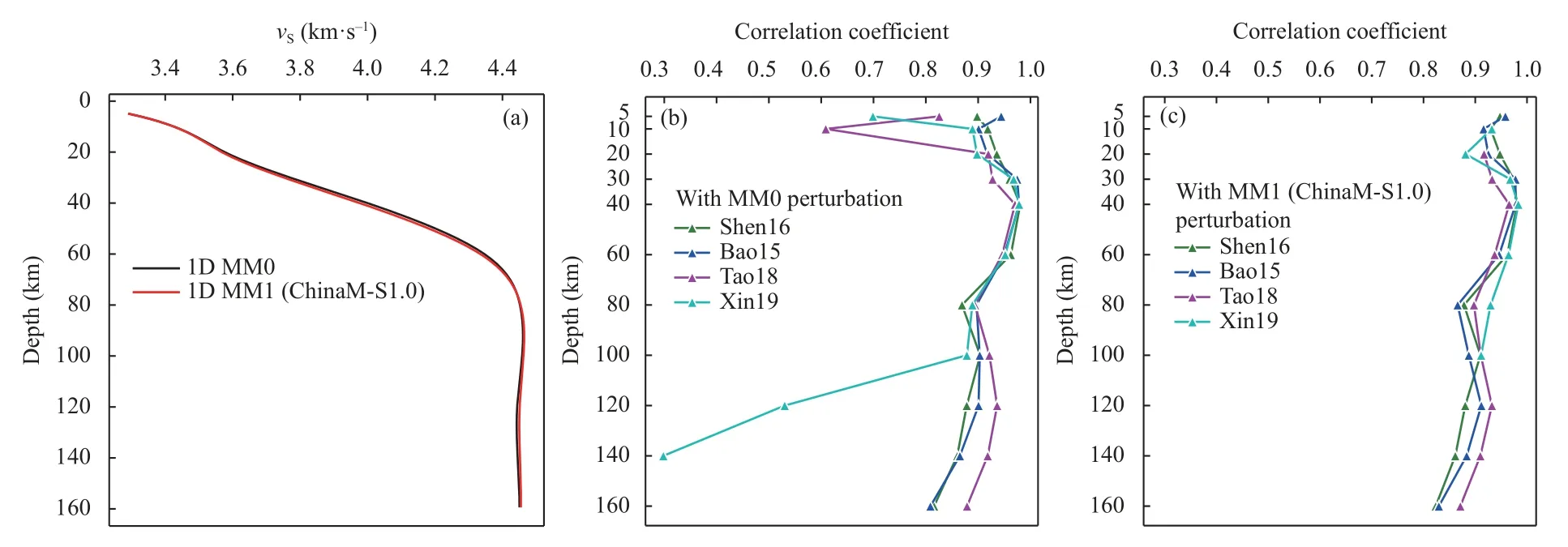
Figure 10.One-dimensional (1D) velocity profiles of an initial merged model (MM0) and the merged model (MM1,‘ChinaM-S1.0’) generated in this study,and CCs between model perturbations and the MM0 and MM1 perturbations.(a)Absolute 1D velocity of MM0 and MM1.(b) CCs of perturbations between each initial candidate perturbation model and MM0 with depth.(c) CCs of perturbations between each retained model and MM1 with depth.

Figure 10c shows the CCs between each retained model and the MM1 with depth.This shows that the retained model has high correlations,indicating it is in good agreement with results for surface waves,body waves,and full waveforms at the corresponding depths.The MM1 model of absolute velocity is the sum of the 1D MM0 and MM1 perturbation at each depth and each grid,yielding 3D MM1 of absolute velocity (‘ChinaM-S1.0’;Figures 11–12).The 1D averaged model of the ChinaMS1.0 model was also calculated,which only shows a small departure from the 1D MM0 absolute velocity profile(Figure 10a).

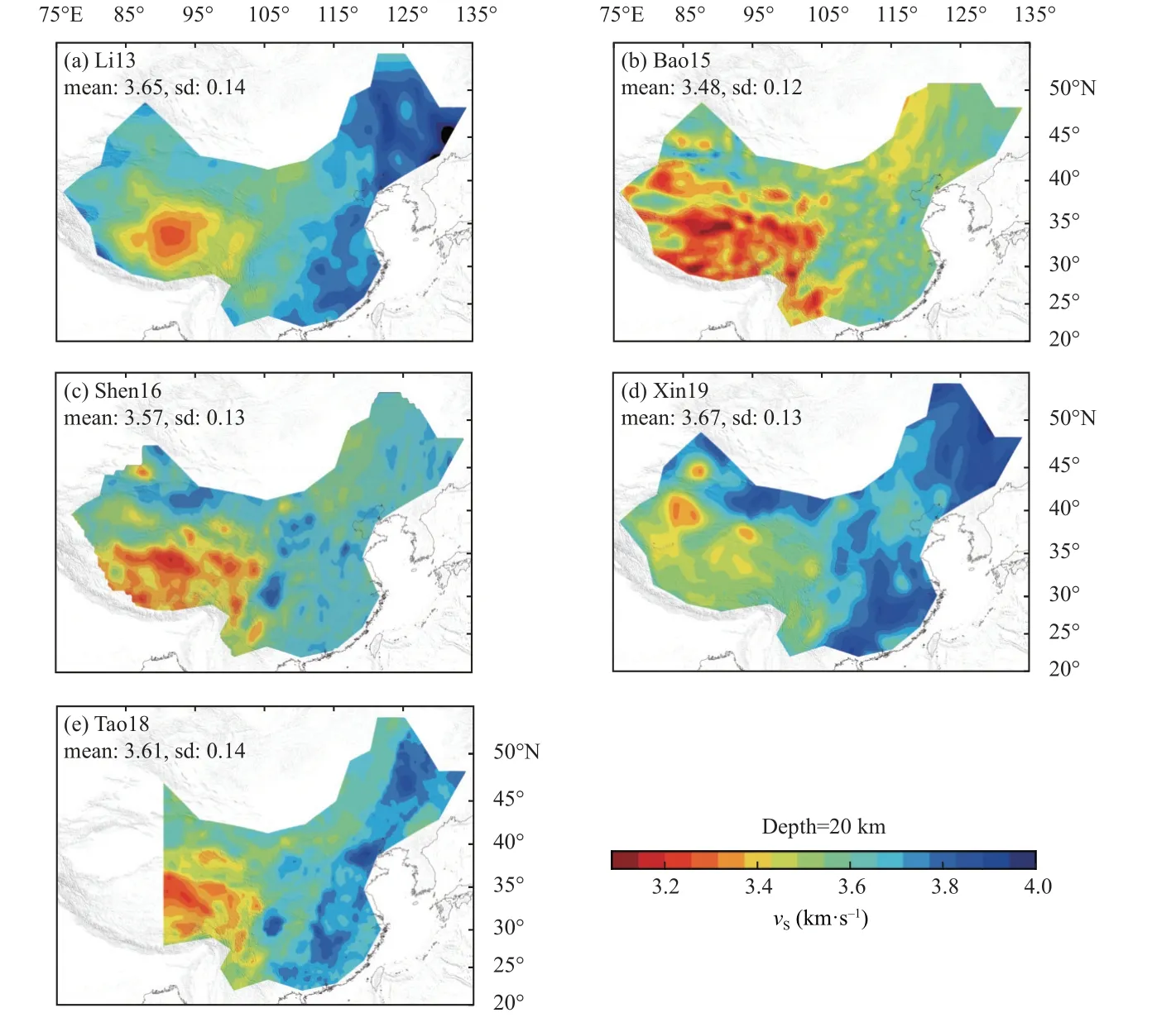
Figure S1.Same as Figure 2 but for five published S-velocity models at 20 km depth.

Figure S2.Same as Figure S1,but at 60 km depth.

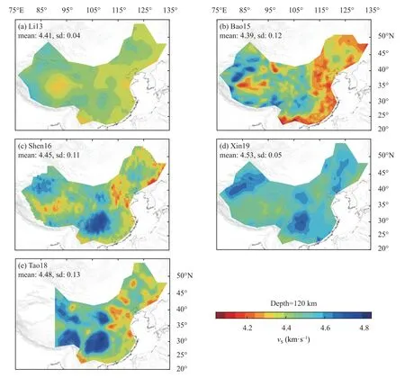
Figure S3.Same as Figure S1,but at 120 km depth.

Figure S4.Same as Figure 3,but at 20 km depth.

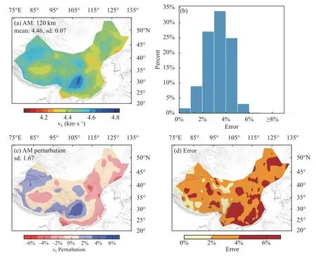
Figure S6.Same as Figure S4,but at 120 km depth.

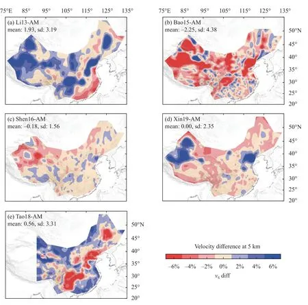
Figure S7.Same as Figure 5,but at 5 km depth.

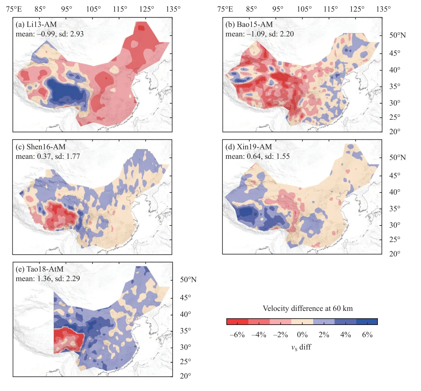
Figure S8.Same as Figure S7,but at 60 km depth.

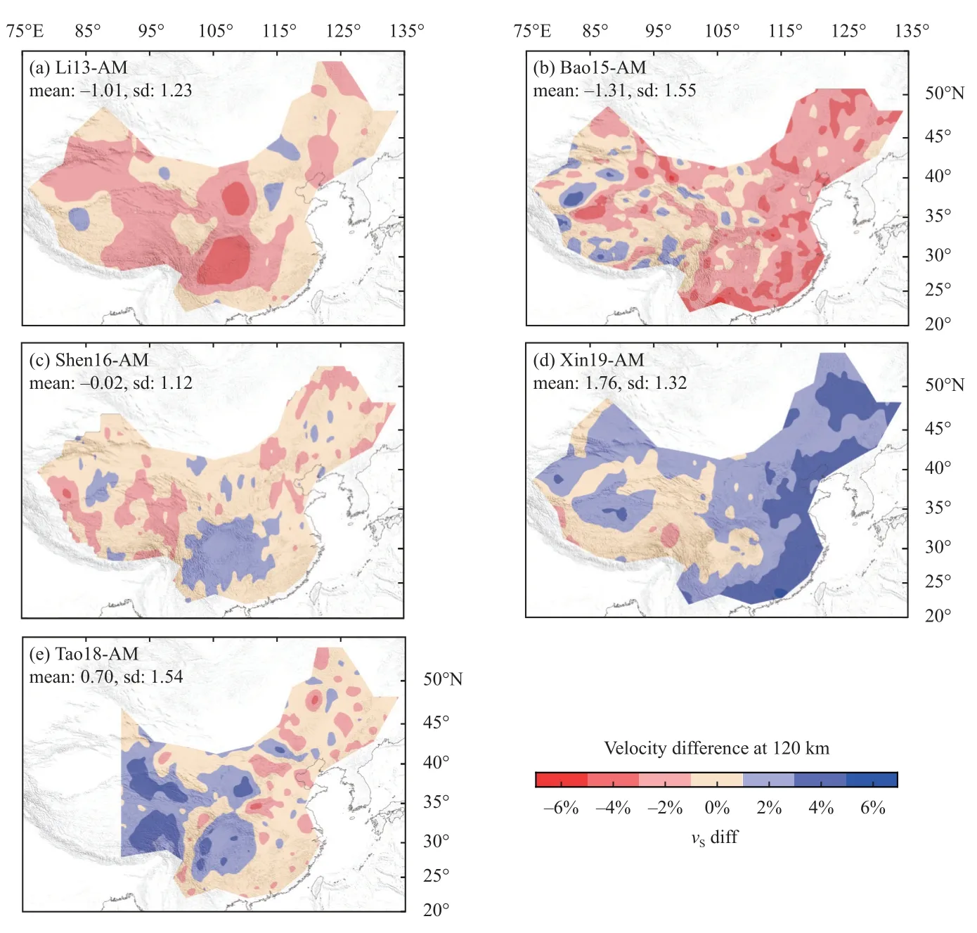
Figure S9.Same as Figure S7,but at 120 km depth.

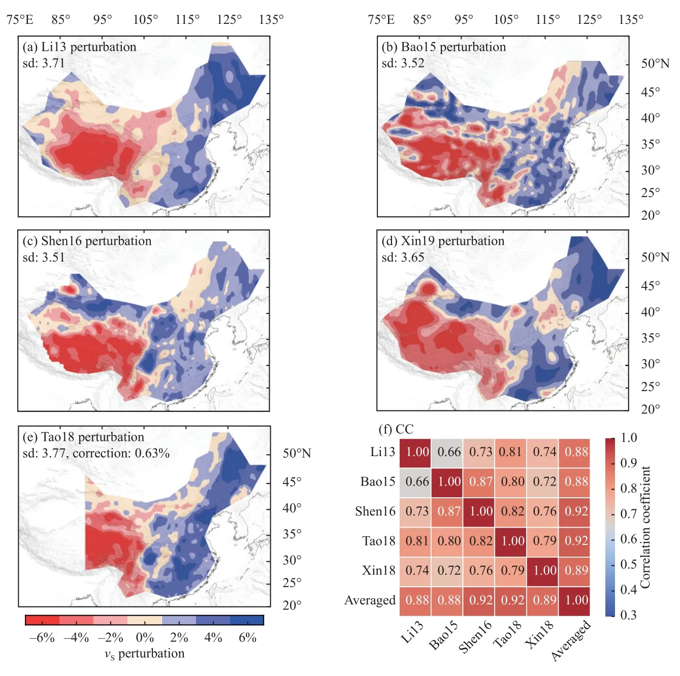
Figure S10.Same as Figure 6,but at 20 km depth.

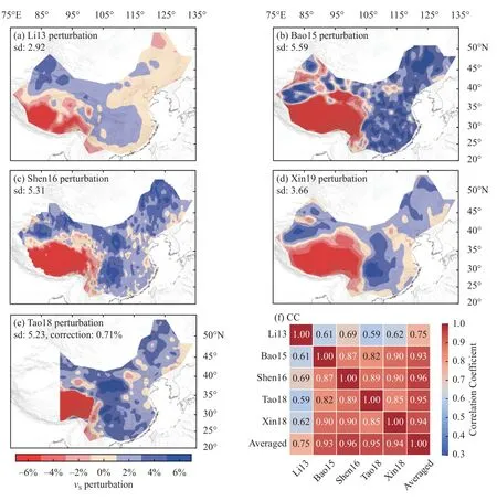
Figure S11.Same as Figure S10,but at 60 km depth.

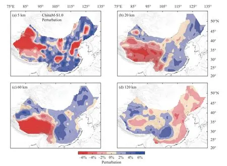
Figure 11.Maps of velocity perturbations generated by the merged model ‘ChinaM-S1.0’ at 5 (a),20 (b),60 (c),and 120 km depths (d).

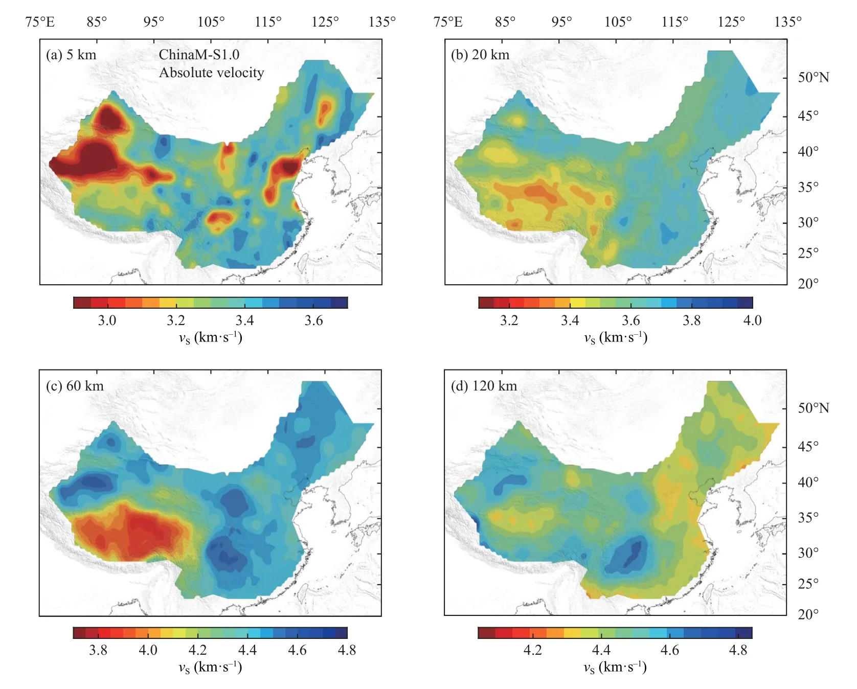
Figure 12.Maps of absolute velocity generated by the merged model ‘ChinaM-S1.0’ at 5 (a),20 (b),60 (c),and 120 km depths (d).

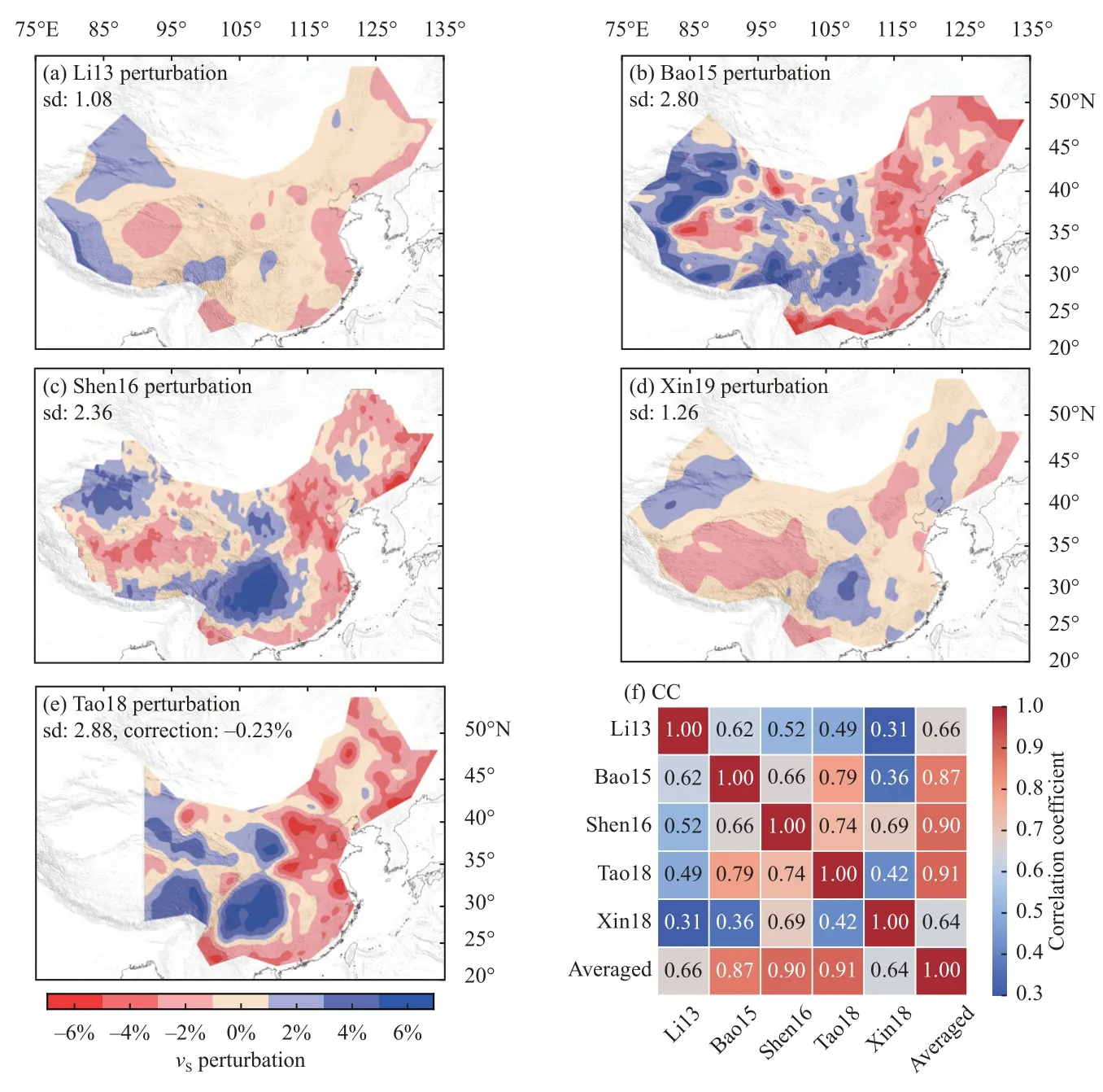
Figure S12.Same as Figure S10,but at 120 km depth.

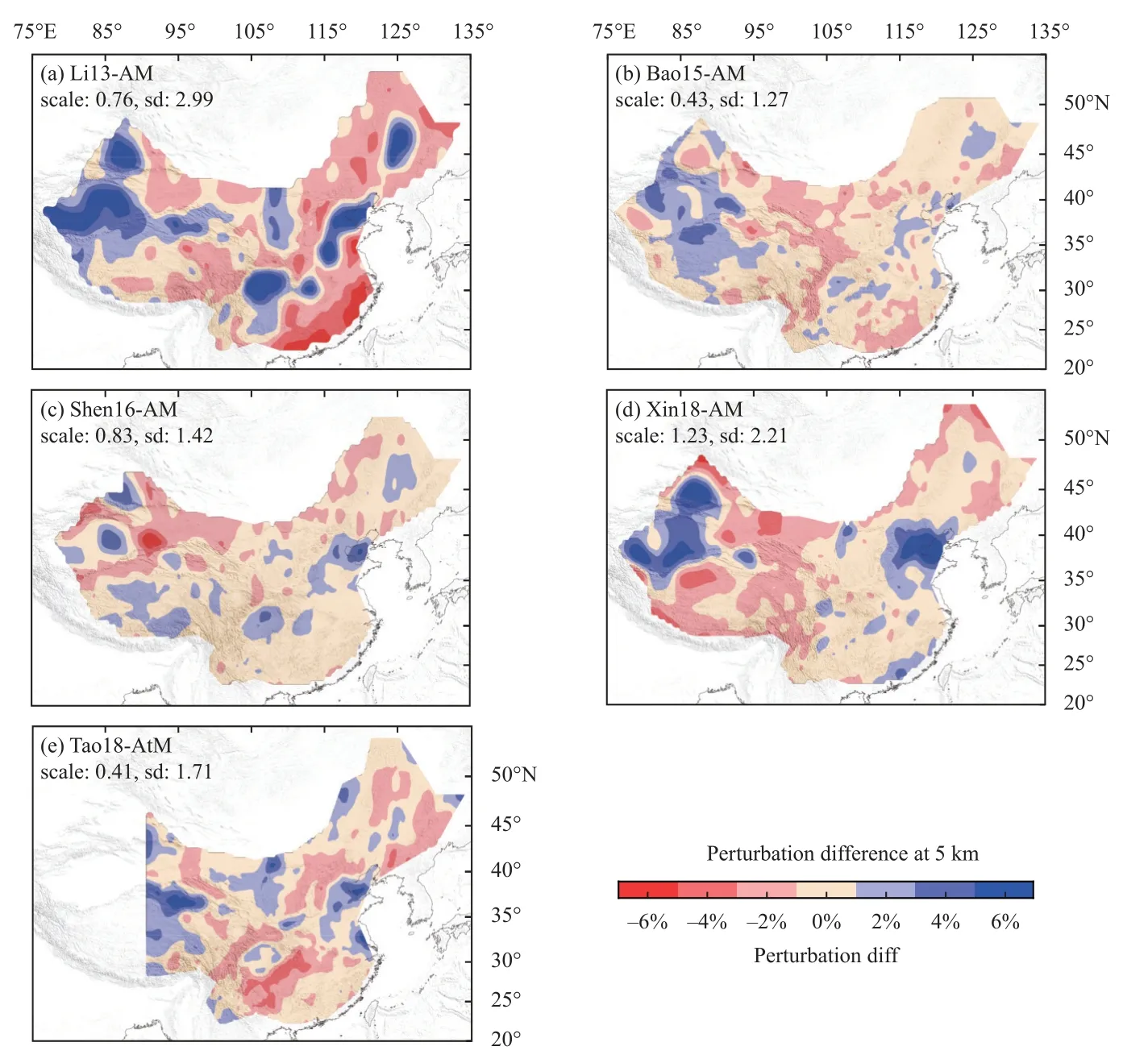
Figure S13.Same as Figure 7,but at 5 km depth.

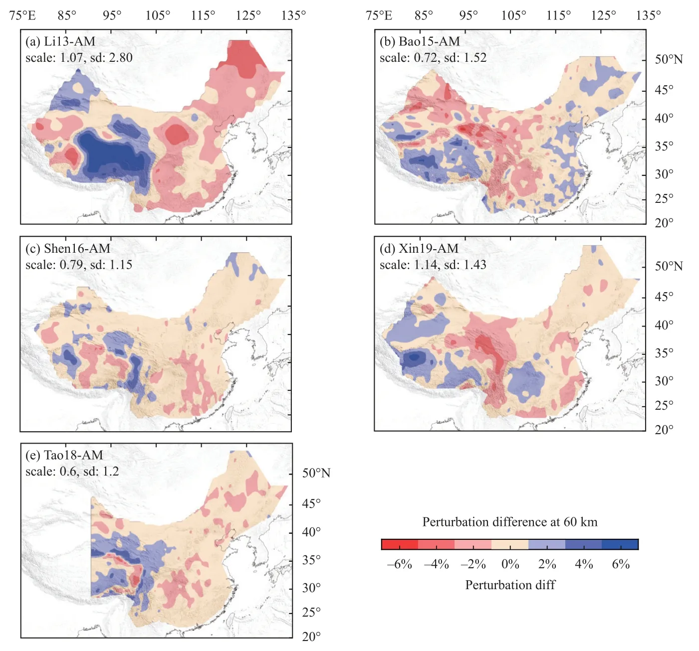
Figure S14.Same as Figure S13,but at 60 km depth.

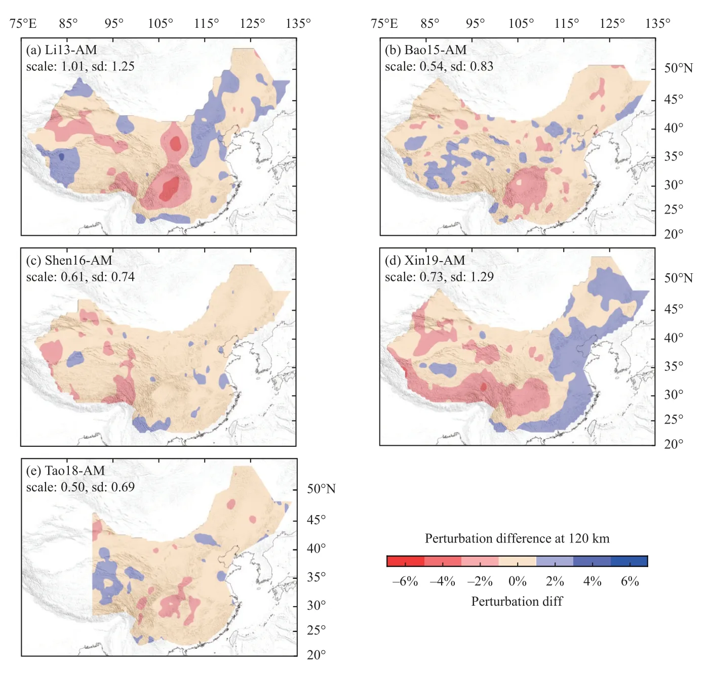
Figure S15.Same as Figure S13,but at 120 km depth.

5.Conclusions

(1) We compared five published S-wave velocity models of the Chinese continental lithosphere,which were derived using different datasets (i.e.,surface waves from noise and earthquakes,body waves,and full waveforms)and different inversion methods.We found large discrepancies among the velocity models,both in absolute values and perturbation patterns.However,the consistency among some of the models is encouraging.

(2) In the case of absolute values,the SDs of the five models exceeded 4% in many places,which is comparable to the amplitudes of the velocity perturbations of each model.We also identified systematic differences between the models (e.g.,in general,velocity values were ranked Tao18 ＞ Shen16 ＞ Bao15) due to systematic discrepancies between noise and event data as well as differences in the datasets and methods employed in their development.

(3) Some of the models produced very different perturbation patterns,such as the Li13 model at almost all depths and the Xin19 model at depths ＞ 100 km.Notably,the model patterns diverge at depths ＜ 10 km.In contrast,three models (Bao15,Shen16,and Tao18) show good consistency at depths ＞10 km;we also found that the Xin19 model is generally consistent with three other models in the 10–100 km depth range.Nevertheless,the amplitudes of the perturbations of the consistent models still differed by up to 100%.

(4) Possible causes of the observed inconsistencies between the models include: ①different data types (i.e.,body waves,surface waves,and full waveforms) and data coverage;② systematic discrepancies between dataset types (e.g.,surface waves from ambient noise and earthquakes);③the different methods employed to develop each model (e.g.,the choice of the starting model and model parameterization,particularly the treatments of discontinuities);and ④ low-resolution data at shallow depth (＜ 10 km).Notably,the amount of data does not appear to be the most important factor affecting the observed discrepancies and,therefore,increasing data coverage may not resolve this issue.The exception is at shallow depths,where the models most likely diverge greatly due to generally poor data coverage and resolution.

(5) We constructed a MM (ChinaM-S1.0) from the five published models based on model consistency,which can serve as a new reference model for the S-wave velocity structure of the Chinese mainland lithosphere.Our merging approach provides a way of extracting the consistent features of existing models and,thus,identifying the robust features of the lithospheric structure.

(6) There is significant room for improvement in the Chinese mainland seismic models.In particular,more effort is needed to resolve the inconsistencies in both the data and methodologies used.For example,as previously stated,systematic discrepancies between data types and possible biases from the choice of starting models and their parameterization need to be addressed.Furthermore,model resolution at shallow depths (＜ 10 km) needs to be significantly improved.This will also help improve model reliability at greater depths due to the trade-off between depth sensitivity of many data types,particularly surface waves.

Data availability

The original digital model data for the five published models examined in this study can be found from the respective publications.In the Supplemental Information,we provide digital model data in a uniform format,including our merged model ChinaM-S1.0 as well as the interpolated versions of the five previously published models.

Acknowledgments

We thank two anonymous reviewers for their constructive and thoughtful comments,which helped improve the manuscript.Most of the figures were generated using Generic Mapping Tools (GMT,Wessel et al.,2019).The China National Seismic Network location data were obtained from the China Earthquake Science Knowledges Service System (http://earthquake.ckcest.cn/).This research was supported by the Special Fund of the Institute of Geophysics,China Earthquake Administration (Grant No.DQJB21B32),and the National Natural Science Foundation of China (No.U1939204).

Supplementary information

Continued

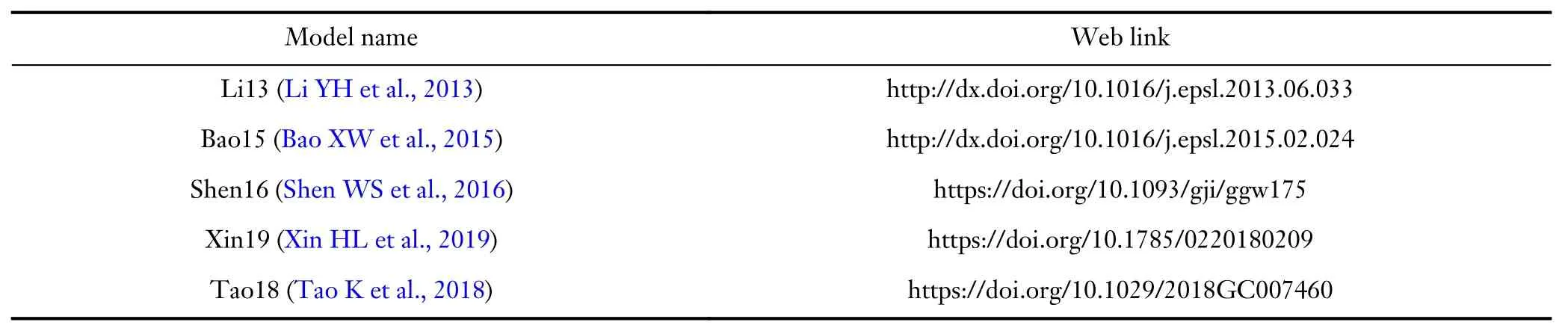
Table S2.Web links of the five models.