Comparing the Soil Conservation Service model with new machine learning algorithms for predicting cumulative infiltration in semi-arid regions

Khabat KHOSRAVIPhuong T.T.NGORahim BARZEGARJohn QUILTYMohammad T.AALAMI and Dieu T.BUI

1Department of Watershed Management Engineering,Ferdowsi Universityof Mashhad,Mashhad 93(Iran)

2Department of Earth and Environment,Florida International University,Miami 33199(USA)

3Institute of Research and Development,DuyTan University,Da Nang 550000(Vietnam)

4Department of Bioresource Engineering,McGill University,Ste Anne de Bellevue QC H9X(Canada)

5Facultyof Civil Engineering,Universityof Tabriz,Tabriz51(Iran)

6Department of Civil and Environmental Engineering,Universityof Waterloo,Waterloo N2L 3G1(Canada)

7Department of Business and IT,Universityof South-Eastern Norway,Notodden 3603(Norway)

ABSTRACT Water infiltration into soil is an important process in hydrologic cycle;however,its measurement is difficult,time-consuming and costly.Empirical and physical models have been developed to predict cumulative infiltration(CI),but are often inaccurate.In this study,several novel standalone machine learning algorithms(M5Prime(M5P),decision stump(DS),and sequential minimal optimization(SMO))and hybrid algorithms based on additive regression(AR)(i.e.,AR-M5P,AR-DS,and AR-SMO)and weighted instance handler wrapper(WIHW)(i.e.,WIHW-M5P,WIHW-DS,and WIHW-SMO)were developed for CI prediction.The Soil Conservation Service(SCS)model developed by the United States Department of Agriculture(USDA),one of the most popular empirical models to predict CI,was considered as a benchmark.Overall,154 measurements of CI(explanatory/input variables)were taken from 16sites in a semi-arid region of Iran(Illam and Lorestan provinces).Six input variable combinations were considered based on Pearson correlations between candidate model inputs(time of measuring and soil bulk density,moisture content,and sand,clay,and silt percentages)and CI.The dataset was divided into two subgroups at random:70%of the data were used for model building(training dataset)and the remaining 30%were used for model validation(testing dataset).The various models were evaluated using different graphical approaches(bar charts,scatter plots,violin plots,and Taylor diagrams)and quantitative measures(root mean square error(RMSE),mean absolute error(MAE),Nash-Sutcliffe efficiency(NSE),and percent bias(PBIAS)).Time of measuring had the highest correlation with CI in the study area.The best input combinations were different for different algorithms.The results showed that all hybrid algorithms enhanced the CI prediction accuracy compared to the standalone models.The AR-M5P model provided the most accurate CI predictions(RMSE=0.75 cm,MAE=0.59 cm,NSE=0.98),while the SCS model had the lowest performance(RMSE=4.77 cm,MAE=2.64 cm,NSE=0.23).The differences in RMSE between the best model(AR-M5P)and the second-best(WIHW-M5P)and worst(SCS)were 40%and 84%,respectively.

KeyWords: additive regression,hybrid algorithms,empirical model,soil water infiltration,weighted instances handler wrapper

INTRODUCTION

Infiltration is the process of water penetrating soil surface and moving into unsaturated soil and is,therefore,an important component of hydrologic cycle.The total amount of water infiltrating into soil in a given time is defined as cumulative infiltration(CI)(Solaimaniet al.,2016).Parameters such as soil texture,density,moisture and hydraulic conductivity,as well as rainfall intensity and land use,control the infiltration process in a watershed(Angelakiet al.,2013).Owing to the importance of infiltration in the water supply for plant growth,groundwater recharge,subsurface and groundwater quality,rainfall-runoffmodeling,flood generation,and design of flood control structures and watershed management plans,it has received much attention in the literature(Angelakiet al.,2018;Singhet al.,2018).Therefore,quantifying CI is important in watershed management.Direct measurement of infiltration is time-consuming,challenging,and costly,especially over large-scale areas.Therefore,an accurate model to predict CI is a useful tool for water resources management.

Various physical equations have been developed for infiltration prediction based on energy and mass conservation laws(Green and Ampt,1911;Richards,1931;Philip,1957a,b).Moreover,numerous empirical infiltration models,including those by Soil Conservation Service(SCS)(1972),Kostiakov(1932),and Horton(1941),were derived based on field and laboratory investigations.Spatio-temporal soil conditions have a significant impact on the accurate estimation of each empirical model’s coefficient(s);this is seen as one of the main drawbacks to these models(Loáiciga and Huang,2007).Other weaknesses include various assumptions made during model development,such as the homogeneity of soil and constant soil moisture content(Singhet al.,2019),as well as neglecting other important input variables that are useful in predicting CI;e.g.,the SCS model includes the time of measuring as an input variable,but neglects soil moisture.

Although some researchers have shown that physical models can provide more accurate CI predictions than empirical models(Loáiciga and Huang,2007),other researchers have found the opposite(Fakheret al.,2013).Hence,there is no universal guideline to show with certainty which model has the best performance.It has been argued that the empirical models thus far developed for estimating CI often provide unreliable predictions owing to their incompatibility with different soil types and land use characteristics at the catchment scale(Babaeiet al.,2018).

Recently,there has been growing interest in the use of artificial intelligence(AI)and machine learning(ML)algorithms to predict complex hydrological processes(Barzegaret al.,2016,2019).Both AI and ML models have strong prediction capabilities,are rapid to develop,are robust to missing data,can accurately model non-linear relationships between variables,and have the ability to handle large amounts of data at different scales(Kisiet al.,2012;Yaseenet al.,2016).Such algorithms have been successfully used for the prediction of infiltration(Sy,2006;Tiwariet al.,2017;Singhet al.,2018).The artificial neural network(ANN)is the most widely used AI algorithm in hydrology(Abrahartet al.,2012).However,ANN has been shown to have slow convergence speed during model training and low generalization performance if the training dataset and/or hyperparameters are not carefully selected(Melesseet al.,2011; Kisiet al.,2012; Choubinet al.,2018).Recently,an adaptive neuro-fuzzy inference system(ANFIS)was developed by integrating ANN with fuzzy logic.ANFIS,as a hybrid algorithm,generally provides higher performance than both ANN and fuzzy logic;however,it is challenging to accurately determine the weights in the membership function,a critical step in developing accurate ANFIS models (Chenet al.,2017).Vandet al.(2018)applied ANFIS,support vector machine(SVM),and random forest(RF)to predict CI and infiltration rates,and found that SVM provided the best performance.The extreme learning machine(ELM),a computationally efficient version of ANN,has been explored in hydrology for numerous applications,such as sediment transport rate prediction in open channels(Ebtehajet al.,2016),local scour depth prediction around pile groups under clear water conditions (Ebtehajet al.,2018),and streamflow forecasting in a semi-arid region(Yaseenet al.,2016).However,given that ELM is a type of neural network,it is better suited to problems where large training datasets are available(unlike in this study).SVM is another popular ML algorithm in hydrology that has been used for pan evaporation modeling(Goyalet al.,2014),the regional analysis of flow duration curve(Vafakhah and Khosrobeigi Bozchaloei,2020),and ensemble prediction of regional droughts(Ganguli and Reddy,2014).However,SVM can be time-consuming to train,since it is susceptible to hyperparameter selection(Ahmadet al.,2018).

Lately,newer ML algorithms have been developed and explored in an attempt to address some of the weaknesses of current/traditional AI and ML methods.For example,Hussain and Khan(2020)found that RFoutperformed both MLP and SVM for monthly river flow forecasting by 17.85%and 33.60%,respectively,in terms of root mean square error(RMSE).Shamshirbandet al.(2020)found that M5 model trees provided better predictions of the standardized streamflow index than SVM and gene expression programming.Taoet al.(2019)proposed a radial basis M5 model tree for daily suspended sediment load(SSL)prediction and demonstrated its superior performance when compared to the classical M5 model tree, response surface method, and ANN for the Trenton Hydrological Station on the Delaware River(USA),with improvements in RMSE of 26.3%,51.6%,and 53.1%,respectively.Khosraviet al.(2019)explored different standalone decision tree algorithms(M5Prime(M5P),random tree,RF,and reduced error pruning tree)and compared their predictive performance with standalone and hybrid ANFIS with metaheuristic algorithms for reference evaporation prediction.The authors showed that standalone decision tree algorithms could outperform standalone ANFIS,whereas hybrid ANFIS-metaheuristic algorithms performed only slightly better than standalone decision tree algorithms;however,the authors used a much larger dataset than that available in this study,which could be a reason why the ANFIS-metaheuristic algorithm provided slightly better performance.An additional advantage of these newer ML methods is that they require fewer parametric settings and are often more robust than traditional ML methods such as ANN,ANFIS,and SVM.Yaseenet al.(2021)compared the predictive power of Gaussian process regression(GPR),M5P,and RFfor infiltration rate prediction for permeable stormwater channels and found that GPR had the best performance,followed by RFand M5P.The performance of RF,M5P,ANN,multiple linear regression(MLR),and the empirical Kostiakov method were compared for infiltration rate prediction in the Kurukshetra district(India)by Singhet al.(2020),who found that RFprovided the best overall performance and the Kostiakov method provided the worst.Sihaget al.(2020) compared SVM,M5P,MLR,general regression neural networks,SCS,and the Kostakov methods for CI prediction in a laboratory setting,and reported that SVM provided the most accurate predictions.Finally,Pahlavan-Radet al.(2020)used MLR and RFto generate predictive spatial maps of soil water infiltration in the Sistan Plain(Iran),and found that both methods provided suitable predictions but RFwas deemed to provide the most realistic maps(upon visual assessment).

In addition to the newer ML models that are now being applied in hydrology,methods such as decision stump(DS)and sequential minimal optimization(SMO)have not been explored in any detail.The DS algorithm,which has a simple tree-based structure(i.e.,it is a‘shallow’rather than a‘deep’tree)that makes it less likely to overfit the training data,has been shown to provide high performance with benchmark data from the UCI(University of California,Irvine)repository(Holte,1993).DS is also often used as a weak learner in ensemble methods(Freund and Schapire,1996).The SMO algorithm(Platt,1999),which is a computationally efficient algorithm that bypasses the time-consuming quadratic programming problem in SVM,was applied for the prediction of surface roughness and compared with decision tree algorithms(Hashmiet al.,2015).The authors found that both algorithms had high performance,whereas SMO was very fast to train.Given the popularity of tree-based and SVM models in hydrology(Raghavendra and Deka,2014;Tyraliset al.,2019),both DS and SMO are relevant algorithms to explore,given their high potential.

Another area of increasing interest in hydrology is hybrid modeling,i.e.,the combination of specialized approaches(e.g.,input pre-processing,ensemble methods)to improve the performance of standalone ML algorithms.In hydrology,different approaches to hybrid ML modeling include metaheuristic optimization (Jinget al., 2019), decomposition(Barzegaret al.,2017; Fijaniet al.,2019),and ensemble methods(e.g.,bagging and boosting)(Zaieret al.,2010).In particular,this study focused on ensemble approaches,given their widespread use in hydrology(Wanget al.,2015;Prasadet al.,2018;Quiltyet al.,2019),by considering two approaches that have not yet been explored in hydrology,additive regression(AR)(Stone,1985)and weighted instance handling wrapper(WIHW)(Morring and Martinez,2004).AR improves the performance of the standalone model by fitting its errors at the previous stage,beginning with the initial predictions of the standalone model.Finally,each ensemble member’s predictions are aggregated to produce the ensemble prediction (Sanz-Garciaet al., 2014). The WIHW method uses weighted instances to generate multiple examples of the training set for each standalone model and combines their results to generate the ensemble prediction.

Most of the above-mentioned studies have demonstrated that newer standalone ML algorithms (M5P,RF,etc.) are promising alternatives to traditional AI and ML methods(ANN,ANFIS,and SVM).Hybrid algorithms can further improve predictive performance over standalone algorithms owing to their increased flexibility(use of multiple models with different parameters).Furthermore,of the more recent ML algorithms mentioned above,only RFand M5P have been applied so far for CI prediction (Singhet al.,2018,2019).Therefore,given their ability to generate accurate predictions for a wide number of hydrological processes,newer standalone and hybrid ML methods are worthwhile alternatives to explore for CI prediction.

The main objective of the current study was to predict CI using new standalone and hybrid ML algorithms,which is an important topic given that there have been few studies exploring such methods for CI prediction and that these studies have reported encouraging results. In this study,three standalone ML algorithms(M5P,DS,and SMO)and six novel hybrid algorithms of AR(i.e.,AR-M5P,AR-DS,and AR-SMO)and WIHW(i.e.,WIHW-M5P,WIHW-DS,and WIHW-SMO)were developed for CI prediction.The predictive performance of each model was evaluated through graphical tools and quantitative measures commonly adopted in hydrology.To demonstrate the utility of the proposed ML algorithms, their results were also compared against an empirical benchmark, the SCS model, developed by the United States Department of Agriculture(USDA).To the best of the authors’ knowledge, the proposed standalone and hybrid algorithms have not been explored in any detail in hydrology or,more generally,in the geosciences (with the exception of M5P).Therefore,the exploration of such methods for hydrological prediction(with CI prediction as a case study)is the main contribution stemming from this study.

MATERIALS AND METHODS

Studyarea

The CI field measurements were taken in a total of 16sites(Table I)with a variety of land uses in two provinces in western Iran:Lorestan(Davood Rashid and Honam areas)and Illam(Kelat region)(see Vandet al.(2018)for further information on the dataset used herein)(Fig.1).The study area has a Mediterranean climate and a mean annual rainfall of about 550 mm(Solaimaniet al.,2016).The maximum and minimum elevations in the study area are 3 300 and 2 100 m,respectively(Behrahiet al.,2018).Most parts of the study area are covered by rangeland; however,dry farming and irrigation land are also prominent.

Dataset collection

Infiltration rate and CI data were collected using a doublering infiltrometer at 16sites(Vandet al.,2018).The doublering had a depth of 30 cm and inner and outer diameters of 30 and 60 cm,respectively.Before starting each experiment,both inner and outer rings were driven 10 cm into the soil.The outer ring prevented leaching from the inner ring,and all measurements were carried out in the inner ring.At first,both rings were filled with water;measurements started with an initial time=0,and measurements were taken at time intervals of 2.5,5,15,20,30,35,40,50,and 70 min until the infiltration rate became steady.A soil sample was collected close to the experimental site to determine soil texture(sand,silt,and clay),bulk density,and moisture content.The infiltration rates were calculated according to the CI value per measured time.Details regarding the data collection can be found in Vandet al.(2018).The gravimetric method was used to calculate soil moisture(SM,%)(Reynolds,1970;Shuklaet al.,2014):

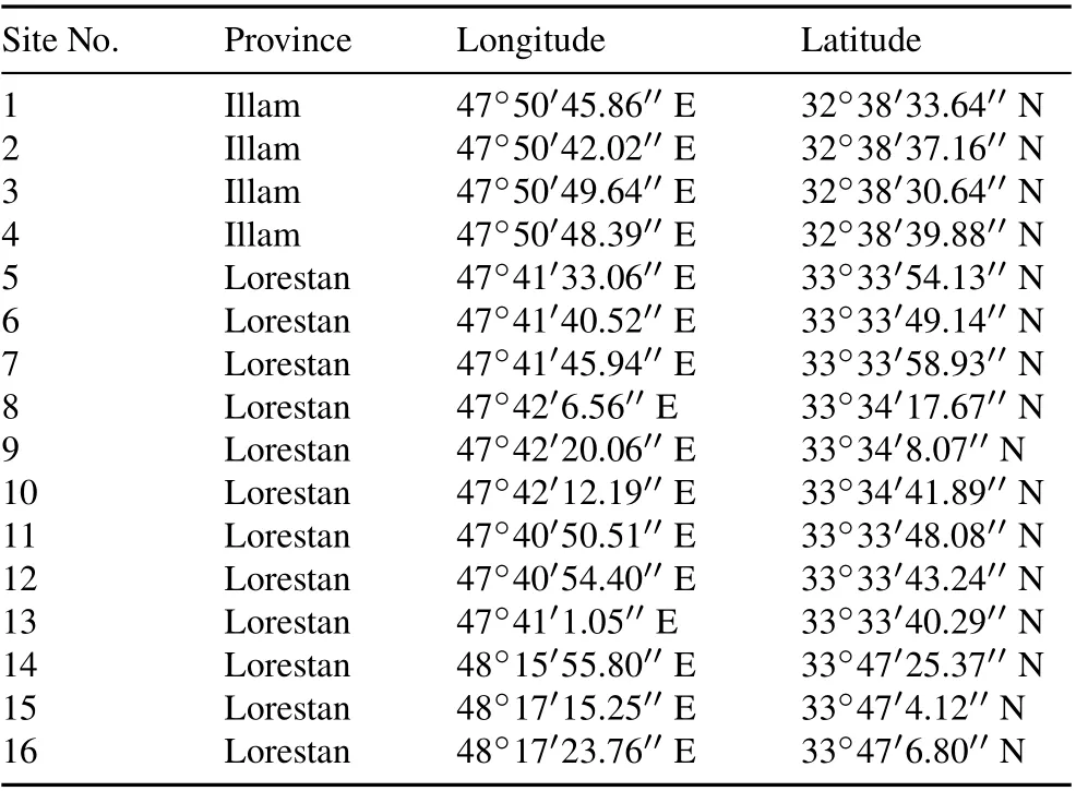
TABLE I Coordinates of 16sites selected,from which cumulative infiltration field measurements were collected,in a semi-arid region(Lorestan and Illam provinces)in western Iran(Vand et al.,2018)

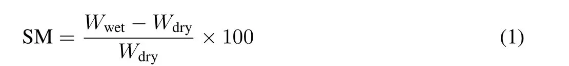
whereWwetandWdryare the wet and dry weights of soil(g),respectively.

Dataset preparation and analysis

The dataset was divided into two subgroups at random:70%was used for model building(training dataset)and 30%for model validation(testing dataset).Although a universal guideline for dividing data into training and testing partitions is lacking,the adopted ratio has been widely used in the literature(Kouadioet al.,2018;Samadianfardet al.,2019).Descriptive statistics of the training and testing datasets are presented in Table II.It can be seen that the CI value varies between 0.3 and 72.1 cm,with a mean value of 23.99 and 23.33 cm for the training and testing sets,respectively.It is observed that silt is the dominant part of the soil samples followed by sand and clay. Importantly, the training and testing datasets have very similar ranges across all variables,which is useful for assessing whether the developed models have strong generalization performance.It is important to note that the available data for all sites were combined into a single dataset to train and evaluate the different models developed in this study.

Input variable selection

The proper selection of input variables is a difficult task in the modeling process and has a significant impact on the predictive performance of the developed model.Pearson correlation coefficients(r)were calculated between the input

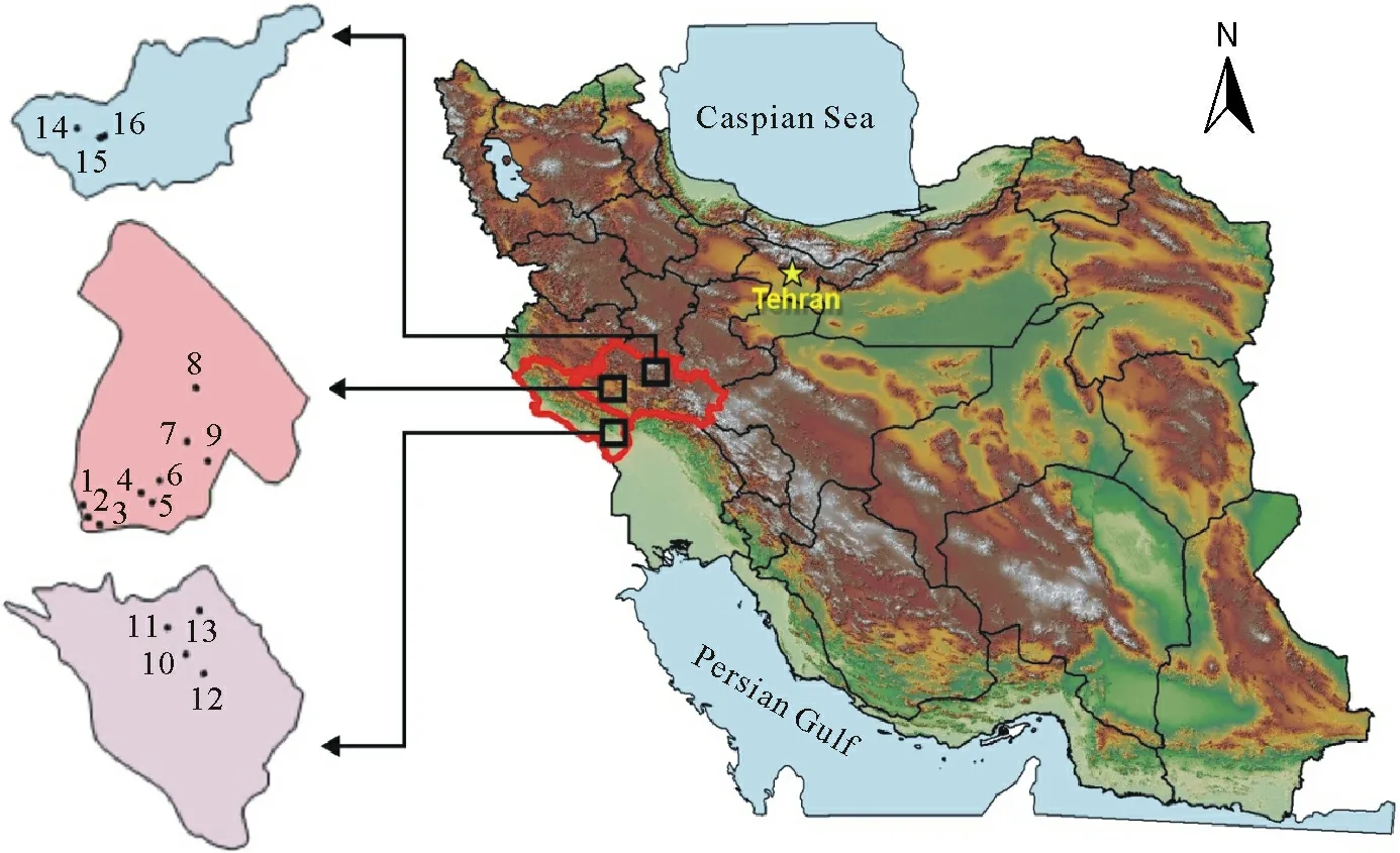
Fig.1 Study area and location of 16sites selected,from which cumulative infiltration field measurements were collected,in a semi-arid region(Lorestan and Illam provinces)in western Iran(Vand et al.,2018).

TABLE II Descriptive statisticsa) of the training and testing datasets

variables and the target(i.e.,CI)(Fig.2)and were used as the basis for selecting different input variable combinations.This is the most common approach in hydrology for selecting which input variables to use in a predictive model(Yaseenet al.,2016;Choubinet al.,2018;Khozaniet al.,2019).

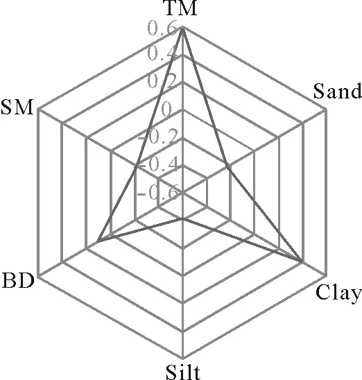
Fig.2 Pearson correlation coefficients between input variables,i.e.,time of measuring(TM)and soil moisture(SM),silt,clay,sand,and bulk density(BD),and cumulative infiltration.

The variable with the highest correlation coefficient was considered the first input to the model (i.e.,time of measuring)to investigate whether or not CI could be estimated with a single(highly correlated)variable.The second input combination was constructed by adding the variable with the next highest correlation coefficient(i.e.,silt).This procedure was continued(i.e.,by successively adding the next of the remaining variables that were most highly correlated with CI)until the variable with the lowest correlation coefficient(i.e.,density)was added(input combination No.6)(Table III).

Each model(M5P,DS,SMO,and their hybrid versions)was paired with the different input variable combinations,and the best performing model(for each model type)was used to identify the optimal input variable combination.Default model hyperparameters were used when determining the optimal input combinations for each model type (see the section below),and RMSE was applied to evaluate the effectiveness of each input variable combination on the training and testing sets. It is important to note that the training and testing datasets each(separately)combined datafrom all sites.Therefore,the correlation coefficients are not site specific but a global estimation of correlation between the different input variables and CI across the entire 16sites.

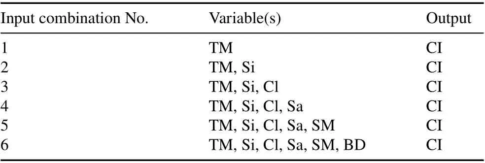
TABLE III Different combinations of input variables,i.e.,time of measuring(TM)and soil moisture(SM),silt(Si),clay(Cl),sand(Sa),and bulk density(BD),used in predicting cumulative infiltration(CI)

Model hyperparameter optimization

Another factor that has a significant impact on the results is identifying the optimal value for each model hyperparameter.Optimal hyperparameter values differ from study to study and there is not an optimum global value;hence,in any study,identifying the optimal model hyperparameters is an important step in the modelbuilding process.Optimal values were determined using the widely accepted trial-and-error approach(Choubinet al.,2018).Models were initially developed using default hyperparameter values and,according to the objective function(RMSE)score,lower or higher values were arbitrarily explored until the objective function was minimized.The RMSE in the training phase was used to identify the optimal hyperparameter values(Table IV).It is worth re-iterating that the optimal model hyperparameters were not site-specific,but were instead estimated by using a dataset that combined all 16sites together.

Models

This section gives a brief description of the empirical(SCS) and ML models developed in this study. All ML models were developed using Waikato Environment for Knowledge Analysis(WEKA)software 3.9(Holmeset al.,1994).

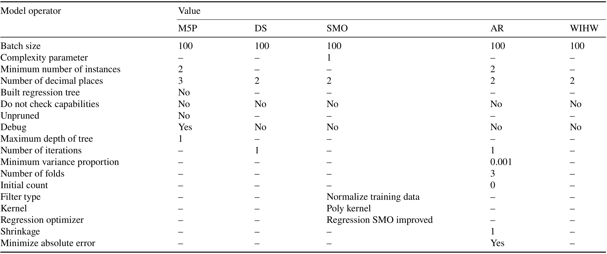
TABLE IV Optimal hyperparameter values for the models used in predicting cumulative infiltration,including standalone machine learning algorithms(M5Prime(M5P),decision stump(DS),and sequential minimal optimization(SMO))and hybrid algorithms based on additive regression(AR)and weighted instances handler wrapper(WIHW)

SCS. The USDA SCS (SCS,1972) found that the

Kostiakov model (Kostiakov, 1932) was not sufficiently accurate for CI prediction.Further experimentation indicated that a coefficient of 0.698 5 was required to improve the Kostiakov model,and a new CI equation was presented as follows(SCS,1972):

whereF(t) is the predicted CI (cm);tis the time (min);andaandbare coefficients that depend on soil type and characteristics.Coefficientsaandbwere determined from measured field data(i.e.,time of measuring and CI)according to the procedure outlined in Kumar and Jain(1982).

M5P.The M5P model is a decision-based tree algorithm which was introduced by Quinlan(1992).The algorithm is a modified version of the M5 algorithm wherein the tree-growing process is the same as that of the classification and regression tree and modifications are introduced during the treepruning process.In constructing the M5P model,three steps(tree construction,tree pruning,and tree smoothing) are considered.Details on these steps can be found in Quinlan(1992).

The M5P model is composed of the reverse tree structure with multivariate regression in which the leaves of the model replace a unique output value with MLR for each subregion.When the model generates branches at nodes,values reaching each node are classified in such a way that the internal variation of the subsets is minimized.When the model is constructed,overfitting is reduced by employing pruning,wherein the inefficient nodes are eliminated (Rodriguez-Galianoet al.,2015).The M5 tree construction process attempts to maximize a measure called the standard deviation reduction (SDR) of the target values of the cases in setTn.Supposing that there is a test tree that splitsTnintoooutcomes,the objective function is used to recognize the potential test tree,calculated as(Linet al.,2016):

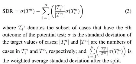
The M5P model is robust,even in the presence of missing data.Moreover,it can use many input variables efficiently(Linet al.,2016;Behnoodet al.,2017).

DS.The DS(Iba and Langley,1992)model is a onelevel decision-tree model that uses only a single variable for splitting.In this model,missing values are treated as a separate variable value and another branch is extended from the stump(Witten and Frank,2002).It also discovers a single variable that can make available the best identification between the variables;then,it bases future predictions on the variable(Iba and Langley,1992;Erdal and Karahanoˇglu,2016).The prediction for categorical or numeric class labels is made using the information-theoretic measure(info(S))represented as follows(Phamet al.,2019):

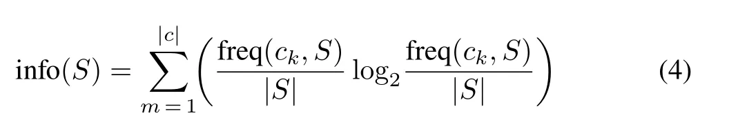
where freq(ck,S)defines the frequency of classckin the training datasetSwith|c| classes.With continuous input variables,the algorithm prioritizes and splits the observed values based on their accuracy scores.This process continues until further divisions no longer increase the gain score,as estimated by the following equation(Kaltonet al.,2001):

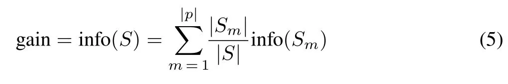
whereSmis a given subset ofS;and|p|is the number of branches.

SMO.The SMO model is an algorithm for solving large quadratic programming (QP) problems in support vector machine(SVM)and was developed by Platt(1999).In the SMO approach,the overall QP problem is broken down into a series of the smallest possible QP sub-problems based on Osuna’s theorem (Osunaet al.,1997) and the overall objective function is decreased at each step where a feasible point that satisfies all of the constraints is retained (Yanget al.,2007).The SMO approach takes advantage of the fact that a QP solver is not needed to solve the problem for the two Lagrange multipliers in SVM since it can be solved analytically.Therefore,numerical QP optimization is avoided entirely(see Platt(1999),Lopezet al.(2012),and Huanget al.(2015)for details).

AR.The AR model adopted here is based on stochastic gradient boosting as presented in Friedman(2002).AR can be summarized as follows:at each iteration,a random sample is drawn from the current training data (without replacement)and a standalone model is fit to the residuals from the previous iteration.Initially,a standalone model is fit to the entire training data(i.e.,no resampling is performed),producing the first set of residuals,which are used in the first iteration of stochastic gradient boosting (i.e.,where resampling is performed)to fit the next standalone model.The stochastic gradient boosting process continues until the final iteration has elapsed. Once an AR model has been trained,model predictions can be obtained by aggregating the predictions of all standalone models in the ensemble,as shown in Friedman(2002).

WIHW.In WIHW, the predictive accuracy of the standalone model is calculated and used as feedback to guide the instance-weighting procedure.In the weighting procedure,a real number is assigned to the distance(e.g.,the Euclidean distance)between the query point(i.e.,a new input variable instance for which a prediction is required)and all training instances such that lower weights cause the target associated with the training instances to influence the model prediction more highly compared to those with higher weights.Essentially,instance weighting adds a higher degree of freedom to the model leading to additional flexibility to model the target variable more accurately.Fig.3 shows how the ensemble algorithms(AR or WIHW)are coupled with standalone algorithms(here as an example,SMO),resulting in the hybrid ML methods.

Fig.3 Flowchart of the methodology of hybrid machine learning algorithms,resulting from additive regression (AR) and weighted instances handler wrapper(WIHW)coupled with sequential minimal optimization(SMO)(modified based on Fig.1 in Lee et al.(2020)).

Model evaluation

Four performance metrics including RMSE,mean absolute error (MAE),Nash-Sutcliffe efficiency (NSE),and percent bias(PBIAS)were used to quantitatively validate the models.The various metrics are calculated as follows:

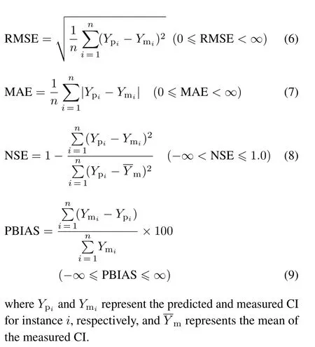
The RMSE and MAE depict the discrepancy between predicted and observed data, with slight differences in how the metrics are determined. They calculate the error/discrepancy in the same units as the predicted output and are therefore easier to interpret(Shiri and Kii,2012).However,RMSE gives more weight to the largest errors,whereas MAE is calculated based on the average magnitude of the error without considering the direction of error.Therefore,RMSE and MAE provide complimentary analyses of model error.The NSE is a dimensionless criterion that allows for the assessment of model performance regardless of the magnitude of the model’s errors.PBIAS calculates the mean tendency of the predicted values with respect to the observed data,reflecting whether predictions are,on average,higher or lower than the observations.

The optimal value for RMSE,MAE,and PBIAS is 0,which represents perfect agreement between the predicted and measured CI,and for NSE,a value of 1 indicates a perfect fit.

In addition to the quantitative evaluation,a visual comparison of the predictedvs. measured CI was explored through bar charts,scatter and violin plots as well as Taylor diagrams.The violin plot summarizes the distribution of each model’s predictions with that of the measured CI through extreme(maximum and minimum)and quartile values(25th,50th(median),and 75th percentiles).The Taylor diagram(Taylor,2001) provides a useful graphical comparison of predicted and measured values;three metrics,comprising correlation coefficient(r),centered RMSE,and the amplitude of their standard deviation,are used simultaneously to show the degree of correspondence between the predicted and measured CI.Unless noted otherwise,the various metrics reported in the text as well as supporting plots and charts are based on the testing dataset.RESULTS AND DISCUSSION

Performance comparison for different input combinations

Input variables that were assumed to have a significant impact on the prediction of CI(time of measuring and soil bulk density,moisture content,and sand,silt,and clay percentages)were considered based on the theory of infiltration,a literature review,and data availability.The results revealed that time of measuring was the input variable most highly correlated to CI(r=0.60)followed by soil silt(r=-0.41),clay(r=0.39),sand(r=-0.22),moisture(r=-0.22),and bulk density(r=0.11).These results were in accordance with those of Sihaget al.(2018)and Singhet al.(2020),who stated that time is the most effective variable for predicting CI.It is important to note that these results are expected to vary from site to site,especially for those sites with different climates and land uses.

The results of the six different input variable combinations that were used when training and evaluating the different models are summarized in Table V.According to the findings,the best input combination for most of the models was input combination No.6(i.e.,the one that considered all input variables).It is noteworthy that both training and testing sets agree on the best performing input combination for each model type.

The optimum input variable combination for SMO,ARSMO,and WIHW-SMO was No.5,and for AR-DS was No.3(Table V).The results revealed that in most cases,models with more input variables had higher prediction accuracy(i.e.,lower RMSE)than those with fewer input variables.This is likely due to the complex and non-linear nature of the infiltration process at the study sites,which cannot be accurately predicted with a low number of variables.Adding more input variables,even those with low correlation coefficients,enhanced the accuracy of the models,since they contained relevant information important to the infiltration process.Additionally, owing to the different structure ofeach ML algorithm, the optimal input combination was not constant across all methods; each standalone model had its own best input variable combination,and certain hybrid algorithms performed best when using the same input variable combination as the standalone algorithms. This result demonstrates that the identification of optimal input variables in standalone algorithms also has a strong effect on the hybrid models.

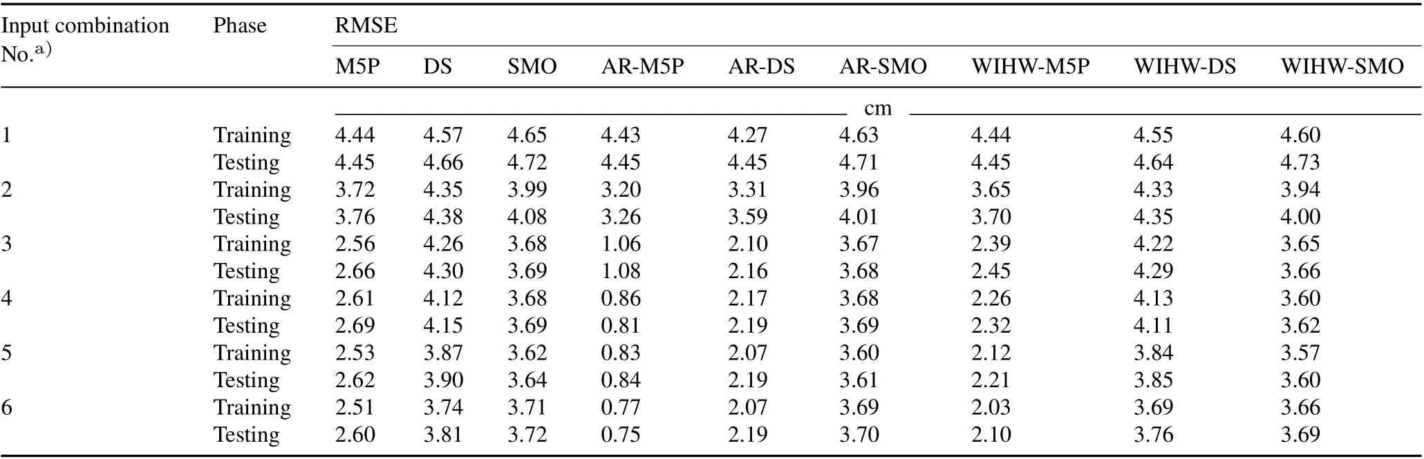
TABLE V Identifying the best input variable combination,used in predicting cumulative infiltration with standalone machine learning algorithms(M5Prime(M5P),decision stump(DS),and sequential minimal optimization(SMO))and hybrid algorithms based on additive regression(AR)(i.e.,AR-M5P,AR-DS,and AR-SMO)and weighted instances handler wrapper(WIHW)(i.e.,WIHW-M5P,WIHW-DS,and WIHW-SMO)according to root mean square error(RMSE)in the testing phase

It is also important to note that certain methods with fewer input variables,although demonstrating slightly lower accuracy,can provide competitive performance with the best performing approaches that include a higher number of input variables.For example,the AR-DS hybrid algorithm with the lowest number of input variables(time of measuring,silt,and clay),provides nearly the same performance as the third-best performing method(WIHW-M5P),which uses all six input variables.Thus,the AR-DS model may be preferred over the WIHW-M5P model(or even over the best performing model AR-M5P,which uses six input variables)based on the concept of parsimony,which becomes very important when collecting data for certain inputs is time-consuming,expensive,and/or difficult(e.g.,soil moisture).Therefore,the different models developed in this study, which, in most cases,incorporate a unique number of input variables,can be very useful tools for decision-makers in real-world scenarios, who need to generate accurate CI predictions based on potentially limited data sources.This finding is not unique to CI prediction for this study area;in general,the accuracy of any predictive model depends on several factors,e.g.,algorithm structure,hyperparameter selection,nature of the data,and size of the dataset(Asimet al.,2018).

Model evaluation and comparison

The various models based on the optimal input variable combinations were then selected for a more thorough analysis of their predictive performance through graphical methods and quantitative measures.Visual comparisons of the predicted and measured CI through bar charts and scatter plots are shown in Figs.4 and 5, respectively. Here, the advantage of the different ML methods is clearly seen;they provide much better performance than the empirical SCS method for high CI values.Among the ML algorithms,the AR-M5P hybrid model had the highest accuracy and DS the lowest.

The violin plots of measured and predicted CI from the nine ML algorithms and the SCS method are shown in Fig.6.The violin plots revealed that AR-M5P predicted the maximum CI value perfectly;AR-SMO predicted it reasonably well,whereas other algorithms performed less well.M5P,SMO,and AR-M5P predicted the minimum value reasonably well,whereas the predictions of other algorithms were poor.M5P,SMO,AR-M5P,AR-SMO,WIHW-M5P,and WIHW-SMO predicted the median CI with high accuracy.

Another important visual approach for model comparison is the Taylor diagram(Fig.7).According to this technique,the hybrid algorithm of AR-M5P outperformed all other algorithms,whereas WIHW-M5P,M5P,and WIHW-SMO showed reasonable performances.The SCS empirical model and DS algorithm produced unsatisfactory results.

The main advantage of these visual comparison approaches is that it is straightforward to recognize which model has the highest and lowest performance; however,the main drawback of these methods is that it is not clear how to rank the various models from best to worst.Hence,quantitative performance criteria are used to generate a ranking of‘model preferences’(Fig.8).According to RMSE(0.75 cm)and MAE(0.59 cm),the hybrid algorithm ARM5P had the highest performance(the lowest RMSE and MAE) for predicting CI.The NSE metric indicated that all algorithms,except for SCS and DS (that had unsatisfactory results),demonstrated good performance(NSE＞0.75)(Moriasiet al.,2007).The SCS model was developed based on specific experimental conditions and regions,using certain assumptions,i.e.,homogeneity of soil and constant soil moisture content(Singhet al.,2019).Additionally,the coefficient of 0.698 5(Eq.2)cannot be considered constant,but varies based on the catchment characteristics.The proper estimation ofaandbcoefficients in Eq.2 is also another source of uncertainty in the SCS empirical equation.The DS algorithm is defined as a one-level decision tree,which is the main drawback of this algorithm.Hence,for the study sites,it needs to be integrated with other ‘compensatory’methods(e.g.,AR or WIHW)to enhance its performance.

According to the NSE values, the hybrid algorithm of AR-M5P (NSE = 0.98) performed best, followed by WIHW-M5P(NSE=0.94),M5P(NSE=0.93),WIHWSMO(NSE=0.85),AR-DS(NSE=0.84),AR-SMO(NSE= 0.81),SMO (NSE = 0.78),WIHW-DS (NSE = 0.75),DS (NSE = 0.26), and SCS (NSE = 0.22).The gain in performance between the best(AR-M5P)and worst(SCS)performing models was 84%,as measured by the RMSE(78%by the MAE).The gain in performance between the best and second-best model(WIHW-M5P)was 40%in terms of RMSE.

The results revealed that although the standalone DS algorithm showed unsatisfactory performance,hybrid algorithms with WIHW and AR could significantly enhance its prediction accuracy(by 35%and 48%,respectively,in terms of RMSE).This finding is also true for two other standalone algorithms(M5P and SMO).For example,AR and WIHW improved the RMSE of M5P(SMO)by 44%(6%)and 7%(15%),respectively.

Fig.4 Bar charts of measured and predicted cumulative infiltration(CI)during the testing phase.The prediction of CI was performed using standalone machine learning algorithms(M5Prime(M5P),decision stump(DS),and sequential minimal optimization(SMO))and hybrid algorithms based on additive regression(AR)(i.e.,AR-M5P,AR-DS,and AR-SMO)and weighted instances handler wrapper(WIHW)(i.e.,WIHW-M5P,WIHW-DS,and WIHW-SMO).An empirical benchmark,the Soil Conservation Service(SCS)model,developed by the United States Department of Agriculture,was used for comparison.

Hybrid algorithms have higher flexibility than standalone algorithms and,in general,they were able to predict CI at the study sites more accurately than the standalone algorithms.This finding is in accordance with those of Khozaniet al.(2019)and Khosraviet al.(2019).Although hybrid algorithms enhanced the prediction accuracy of standalone algorithms,they do not always have a better performance than standalone algorithms.The performance of hybrid algorithms is highly dependent on the base algorithm.For example,the standalone M5P algorithm had a higher performance than the hybrid algorithms of WIHW-SMO and AR-DS.The PBIAS showed that SMO,AR-DS,AR-SMO,and WIHW-DS overestimated CI,whereas other models underestimated it.

The AR model was able to enhance the prediction power of the two standalone algorithms M5P and DS much better than WIHW,whereas the results for the SMO algorithm were the opposite.Therefore,it is not possible to draw a general conclusion that one hybrid algorithm is better than another,which supports the practice of developing a wide range of hybrid models to determine the most suitable approach for a given application.

Fig.5 Scatter plots of measured and predicted cumulative infiltration(CI)during the testing phase.The predicted CI was performed with standalone machine learning algorithms(M5Prime(M5P),decision stump(DS),and sequential minimal optimization(SMO))and hybrid algorithms based on additive regression(AR)(i.e.,AR-M5P,AR-DS,and AR-SMO)and weighted instances handler wrapper(WIHW)(i.e.,WIHW-M5P,WIHW-DS,and WIHW-SMO).An empirical benchmark,the Soil Conservation Service(SCS)model,developed by the United States Department of Agriculture,was used for comparison.

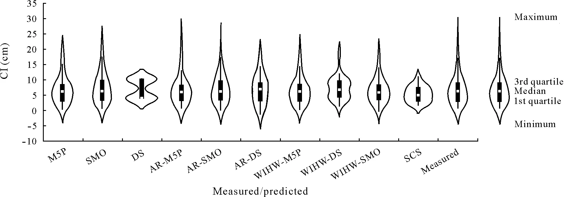
Fig.6 Violin plots of measured and predicted cumulative infiltration(CI)during the testing phase The predicted CI was performed with standalone machine learning algorithms(M5Prime(M5P),decision stump(DS),and sequential minimal optimization(SMO))and hybrid algorithms based on additive regression(AR) (i.e.,AR-M5P,AR-DS,and AR-SMO) and weighted instances handler wrapper (WIHW)(i.e.,WIHW-M5P,WIHW-DS,and WIHW-SMO).An empirical benchmark,the Soil Conservation Service(SCS)model,developed by the United States Department of Agriculture,was used for comparison.

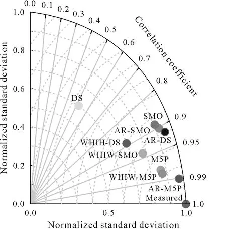
Fig.7 Taylor diagram for the evaluation of model performance for cumulative infiltration prediction.The models used included standalone machine learning algorithms(M5Prime(M5P),decision stump(DS),and sequential minimal optimization (SMO)) and hybrid algorithms based on additive regression(AR)(i.e.,AR-M5P,AR-DS,and AR-SMO)and weighted instances handler wrapper (WIHW) (i.e., WIHW-M5P, WIHW-DS, and WIHW-SMO).An empirical benchmark,the Soil Conservation Service(SCS)model,developed by the United States Department of Agriculture,was used for comparison.

Finally,to demonstrate the site-specific performance of the different models,the CI prediction for each method was plotted as a function of time for site No.1(Fig.9).It can be seen that AR-M5P,WIHW-M5P,M5P,and WIHW-SMO were able to predict CI very accurately as a function of time,providing a highly accurate alternative to the conventional SCS model,whereas DS and WIHW-DS had unsatisfactory predictions when examined as a function of time.According to Fig.9,the SCS model underestimated CI when studied as a function of time.

As the ML algorithms applied in this study have not been explored in great detail,i.e.,not only for CI prediction but also for other hydrological modeling applications, a direct comparison with other studies was not straightforward.However,through a literature review,it was found that Singhet al.(2018,2019)and Vandet al.(2018)applied different algorithms to CI and infiltration rate prediction using different machine learning algorithms,including Gaussian process(NSE=0.75),gene expression programming(NSE=0.63),ANFIS(NSE=0.85),SVM(NSE=0.92),and RF(NSE=0.96),and both studies used the same data adopted herein.The results of the hybrid AR-M5P model presented herein demonstrates an improvement in NSE of 2%–56% when compared to these earlier results.

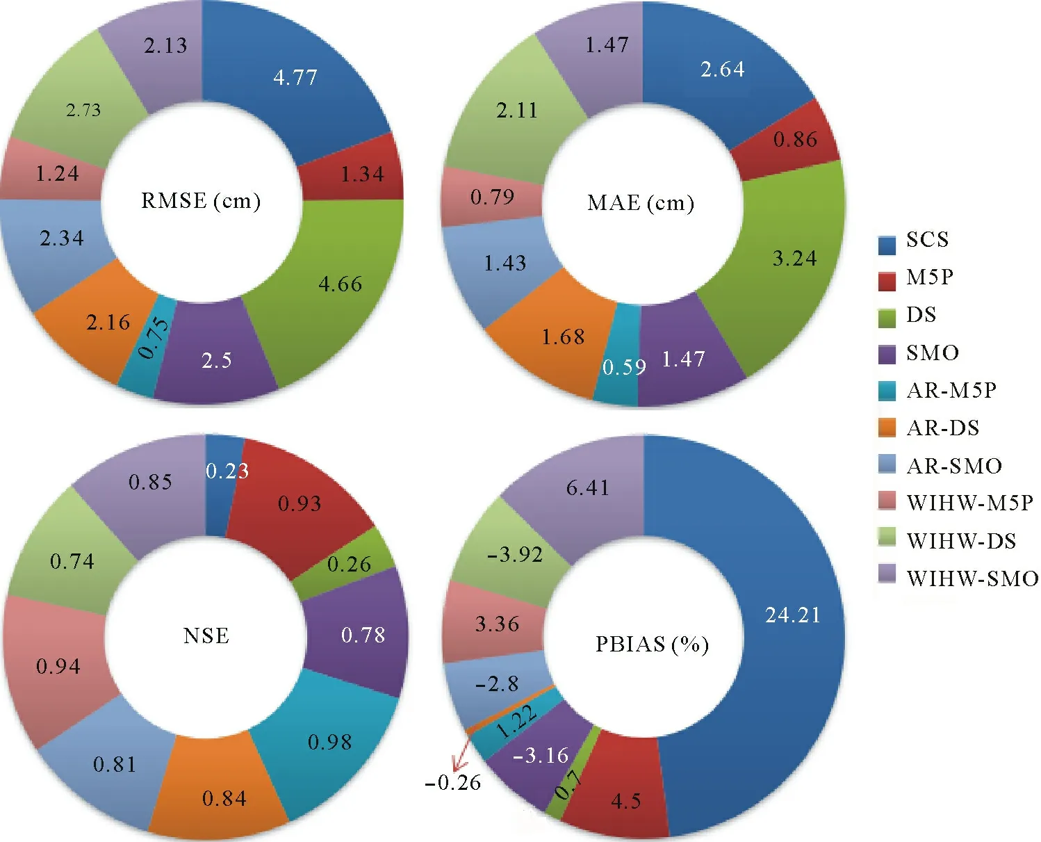
Fig.8 Doughnut charts for the evaluation of model performance for cumulative infiltration prediction using quantitative metrics including root mean square error(RMSE),mean absolute error(MAE),Nash-Sutcliffe efficiency(NSE),and percentage of bias(PBIAS),during the testing phase.The models used included standalone machine learning algorithms(M5Prime(M5P),decision stump(DS),and sequential minimal optimization(SMO))and hybrid algorithms based on additive regression(AR)(i.e.,AR-M5P,AR-DS,and AR-SMO)and weighted instances handler wrapper(WIHW)(i.e.,WIHW-M5P,WIHW-DS,and WIHW-SMO).

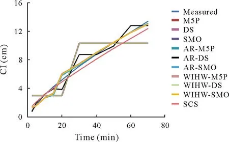
Fig.9 Measured and predicted cumulative infiltration(CI)over time for site No.1.The prediction of CI was performed using standalone machine learning algorithms(M5Prime(M5P),decision stump(DS),and sequential minimal optimization (SMO)) and hybrid algorithms based on additive regression(AR)(i.e.,AR-M5P,AR-DS,and AR-SMO)and weighted instances handler wrapper (WIHW) (i.e., WIHW-M5P, WIHW-DS, and WIHW-SMO).An empirical benchmark,the Soil Conservation Service(SCS)model,developed by the United States Department of Agriculture,was used for comparison.

It is important to note that there are several sources of uncertainty with respect to the models developed in this study,including:1)the relatively small sample size stemming from a single study area,2)the sizes of the training and testing sets,3)the randomized splitting of data into training and testing sets, and 4) the uncertainty in input data, input variable selection,model structure,parameters,and model output.Ideas for addressing these issues include:1)gathering data from additional sites and assessing the developed models’prediction performance at these sites(i.e.,spatial validation),and/or using data from additional sites to redevelop the models and improve their robustness for predicting additional conditions not present in the training data,2)building models for various training and testing set sizes,3) applying the robust(but computationally demanding)protocol for creating unbiased training and testing sets(Zhenget al.,2018),and 4)casting the models developed herein within a stochastic data-driven framework(Quilty and Adamowski,2020)that can be used to holistically account for input data, input variable selection,parameter,and model output uncertainty(among other potential sources).

Finally,some promising future research directions include: 1) applying the ML algorithms developed in this study to other sites with potentially different hydrologic conditions,along with a more detailed evaluation of these algorithms in comparison with a broader range of empirical(e.g.,Horton’s method),physical(e.g.,Green-Ampt model),and emerging ML (e.g.,deep learning) models,2) using metaheuristic algorithms to optimize the empirical equation for CI prediction,and 3)using other potentially useful input variables,such as water level above the surface and degree of soil compaction,for CI modeling.

CONCLUSIONS

In this study,three standalone and six novel hybrid ML algorithms were introduced and used to predict CI in a semiarid region of Iran.The results were compared to those of the SCS model,one of the most popular empirical models used to predict CI.Overall,the ML algorithms demonstrated considerably higher performance than the empirical SCS model; the best ML algorithm, AR-M5P, improved the RMSE and MAE by 84%and 78%,respectively,over the SCS model. In general, the hybrid algorithms enhanced the CI prediction accuracy compared to the standalone ML algorithms.Different input variable combinations led to a high variance in ML model performance;e.g.,the best(ARM5P)and second-best(WIHW-M5P)models,which differed by a single input variable,varied in RMSE by 40%.The time of measuring was estimated to have the highest correlation with CI,followed by soil silt,clay,sand,moisture,and bulk density.Our results suggest that these proposed hybrid ML algorithms(AR-M5P,in particular)could be used as highly accurate methods for CI prediction in semi-arid regions in Iran and may also be worthwhile to consider in other parts of the world, as well as for other hydrological modeling applications.

ACKNOWLEDGEMENT

We would like to thank the Editor and two anonymous reviewers for their very useful feedback on the initial manuscript,which helped to significantly improve the quality of this paper.